针对在ojAlgo中将两个矩阵或PrimitiveDenseStores进行元素相乘和两个矩阵元素对应相乘lingo这两个问题,本篇文章进行了详细的解答,同时本文还将给你拓展Anoverviewofg
针对在ojAlgo中将两个矩阵或PrimitiveDenseStores进行元素相乘和两个矩阵元素对应相乘lingo这两个问题,本篇文章进行了详细的解答,同时本文还将给你拓展An overview of gradient descent optimization algorithms、An universal algorithm design of fixed length substring locating、BP neural network optimized by PSO algorithm on Ammunition storage reliability prediction 阅读笔记、c# – Google Drive SDK System.Net.Http.Primitives版本1.5.0.0而不是2.1.10.0等相关知识,希望可以帮助到你。
本文目录一览:- 在ojAlgo中将两个矩阵或PrimitiveDenseStores进行元素相乘(两个矩阵元素对应相乘lingo)
- An overview of gradient descent optimization algorithms
- An universal algorithm design of fixed length substring locating
- BP neural network optimized by PSO algorithm on Ammunition storage reliability prediction 阅读笔记
- c# – Google Drive SDK System.Net.Http.Primitives版本1.5.0.0而不是2.1.10.0
")
在ojAlgo中将两个矩阵或PrimitiveDenseStores进行元素相乘(两个矩阵元素对应相乘lingo)
谁能告诉我如何在ojAlgo中将两个矩阵的对应元素相乘?寻找块函数c[i][j] = a[i][j] * b[i][j]
答案1
小编典典有几种方法可以做到这一点。这是一种选择:
matrixA.operateOnMatching(MULTIPLY,matrixB).supplyTo(matrixC);
MULTIPLY来自静态导入的位置(org.ojalgo.function.constant.PrimitiveMath)。

An overview of gradient descent optimization algorithms
An overview of gradient descent optimization algorithms
Note: If you are looking for a review paper, this blog post is also available as an article on arXiv.
Table of contents:
- Gradient descent variants
- Batch gradient descent
- Stochastic gradient descent
- Mini-batch gradient descent
- Challenges
- Gradient descent optimization algorithms
- Momentum
- Nesterov accelerated gradient
- Adagrad
- Adadelta
- RMSprop
- Adam
- Visualization of algorithms
- Which optimizer to choose?
- Parallelizing and distributing SGD
- Hogwild!
- Downpour SGD
- Delay-tolerant Algorithms for SGD
- TensorFlow
- Elastic Averaging SGD
- Additional strategies for optimizing SGD
- Shuffling and Curriculum Learning
- Batch normalization
- Early Stopping
- Gradient noise
- Conclusion
- References
Gradient descent is one of the most popular algorithms to perform optimization and by far the most common way to optimize neural networks. At the same time, every state-of-the-art Deep Learning library contains implementations of various algorithms to optimize gradient descent (e.g.lasagne''s, caffe''s, and keras'' documentation). These algorithms, however, are often used as black-box optimizers, as practical explanations of their strengths and weaknesses are hard to come by.
This blog post aims at providing you with intuitions towards the behaviour of different algorithms for optimizing gradient descent that will help you put them to use. We are first going to look at the different variants of gradient descent. We will then briefly summarize challenges during training. Subsequently, we will introduce the most common optimization algorithms by showing their motivation to resolve these challenges and how this leads to the derivation of their update rules. We will also take a short look at algorithms and architectures to optimize gradient descent in a parallel and distributed setting. Finally, we will consider additional strategies that are helpful for optimizing gradient descent.
Gradient descent is a way to minimize an objective function J(θ)J(θ) parameterized by a model''s parameters θ∈Rdθ∈Rd by updating the parameters in the opposite direction of the gradient of the objective function ∇θJ(θ)∇θJ(θ) w.r.t. to the parameters. The learning rate ηη determines the size of the steps we take to reach a (local) minimum. In other words, we follow the direction of the slope of the surface created by the objective function downhill until we reach a valley. If you are unfamiliar with gradient descent, you can find a good introduction on optimizing neural networks here.
Gradient descent variants
There are three variants of gradient descent, which differ in how much data we use to compute the gradient of the objective function. Depending on the amount of data, we make a trade-off between the accuracy of the parameter update and the time it takes to perform an update.
Batch gradient descent
Vanilla gradient descent, aka batch gradient descent, computes the gradient of the cost function w.r.t. to the parameters θθ for the entire training dataset:
θ=θ−η⋅∇θJ(θ)θ=θ−η⋅∇θJ(θ).
As we need to calculate the gradients for the whole dataset to perform just one update, batch gradient descent can be very slow and is intractable for datasets that don''t fit in memory. Batch gradient descent also doesn''t allow us to update our model online, i.e. with new examples on-the-fly.
In code, batch gradient descent looks something like this:
for i in range(nb_epochs):
  params_grad = evaluate_gradient(loss_function, data, params)
  params = params - learning_rate * params_grad
For a pre-defined number of epochs, we first compute the gradient vector params_grad of the loss function for the whole dataset w.r.t. our parameter vector params. Note that state-of-the-art deep learning libraries provide automatic differentiation that efficiently computes the gradient w.r.t. some parameters. If you derive the gradients yourself, then gradient checking is a good idea. (See here for some great tips on how to check gradients properly.)
We then update our parameters in the direction of the gradients with the learning rate determining how big of an update we perform. Batch gradient descent is guaranteed to converge to the global minimum for convex error surfaces and to a local minimum for non-convex surfaces.
Stochastic gradient descent
Stochastic gradient descent (SGD) in contrast performs a parameter update for each training example x(i)x(i) and label y(i)y(i):
θ=θ−η⋅∇θJ(θ;x(i);y(i))θ=θ−η⋅∇θJ(θ;x(i);y(i)).
Batch gradient descent performs redundant computations for large datasets, as it recomputes gradients for similar examples before each parameter update. SGD does away with this redundancy by performing one update at a time. It is therefore usually much faster and can also be used to learn online.
SGD performs frequent updates with a high variance that cause the objective function to fluctuate heavily as in Image 1.
 Image 1: SGD fluctuation (Source:
Wikipedia)
Image 1: SGD fluctuation (Source:
Wikipedia)
While batch gradient descent converges to the minimum of the basin the parameters are placed in, SGD''s fluctuation, on the one hand, enables it to jump to new and potentially better local minima. On the other hand, this ultimately complicates convergence to the exact minimum, as SGD will keep overshooting. However, it has been shown that when we slowly decrease the learning rate, SGD shows the same convergence behaviour as batch gradient descent, almost certainly converging to a local or the global minimum for non-convex and convex optimization respectively.
Its code fragment simply adds a loop over the training examples and evaluates the gradient w.r.t. each example. Note that we shuffle the training data at every epoch as explained in this section.
for i in range(nb_epochs):
  np.random.shuffle(data)for example in data:
    params_grad = evaluate_gradient(loss_function, example, params)
    params = params - learning_rate * params_grad
Mini-batch gradient descent
Mini-batch gradient descent finally takes the best of both worlds and performs an update for every mini-batch of nn training examples:
θ=θ−η⋅∇θJ(θ;x(i:i+n);y(i:i+n))θ=θ−η⋅∇θJ(θ;x(i:i+n);y(i:i+n)).
This way, it a) reduces the variance of the parameter updates, which can lead to more stable convergence; and b) can make use of highly optimized matrix optimizations common to state-of-the-art deep learning libraries that make computing the gradient w.r.t. a mini-batch very efficient. Common mini-batch sizes range between 50 and 256, but can vary for different applications. Mini-batch gradient descent is typically the algorithm of choice when training a neural network and the term SGD usually is employed also when mini-batches are used. Note: In modifications of SGD in the rest of this post, we leave out the parameters x(i:i+n);y(i:i+n)x(i:i+n);y(i:i+n) for simplicity.
In code, instead of iterating over examples, we now iterate over mini-batches of size 50:
for i in range(nb_epochs):
  np.random.shuffle(data)for batch in get_batches(data, batch_size=50):
    params_grad = evaluate_gradient(loss_function, batch, params)
    params = params - learning_rate * params_grad
Challenges
Vanilla mini-batch gradient descent, however, does not guarantee good convergence, but offers a few challenges that need to be addressed:
Choosing a proper learning rate can be difficult. A learning rate that is too small leads to painfully slow convergence, while a learning rate that is too large can hinder convergence and cause the loss function to fluctuate around the minimum or even to diverge.
Learning rate schedules [11] try to adjust the learning rate during training by e.g. annealing, i.e. reducing the learning rate according to a pre-defined schedule or when the change in objective between epochs falls below a threshold. These schedules and thresholds, however, have to be defined in advance and are thus unable to adapt to a dataset''s characteristics [10].
Additionally, the same learning rate applies to all parameter updates. If our data is sparse and our features have very different frequencies, we might not want to update all of them to the same extent, but perform a larger update for rarely occurring features.
Another key challenge of minimizing highly non-convex error functions common for neural networks is avoiding getting trapped in their numerous suboptimal local minima. Dauphin et al. [19] argue that the difficulty arises in fact not from local minima but from saddle points, i.e. points where one dimension slopes up and another slopes down. These saddle points are usually surrounded by a plateau of the same error, which makes it notoriously hard for SGD to escape, as the gradient is close to zero in all dimensions.
Gradient descent optimization algorithms
In the following, we will outline some algorithms that are widely used by the deep learning community to deal with the aforementioned challenges. We will not discuss algorithms that are infeasible to compute in practice for high-dimensional data sets, e.g. second-order methods such asNewton''s method.
Momentum
SGD has trouble navigating ravines, i.e. areas where the surface curves much more steeply in one dimension than in another [1], which are common around local optima. In these scenarios, SGD oscillates across the slopes of the ravine while only making hesitant progress along the bottom towards the local optimum as in Image 2.
 Image 2: SGD without momentum Image 2: SGD without momentum |
 Image 3: SGD with momentum Image 3: SGD with momentum |
Momentum [2] is a method that helps accelerate SGD in the relevant direction and dampens oscillations as can be seen in Image 3. It does this by adding a fraction γγ of the update vector of the past time step to the current update vector:
vt=γvt−1+η∇θJ(θ)vt=γvt−1+η∇θJ(θ).
θ=θ−vtθ=θ−vt.
Note: Some implementations exchange the signs in the equations. The momentum term γγ is usually set to 0.9 or a similar value.
Essentially, when using momentum, we push a ball down a hill. The ball accumulates momentum as it rolls downhill, becoming faster and faster on the way (until it reaches its terminal velocity if there is air resistance, i.e. γ<1γ<1). The same thing happens to our parameter updates: The momentum term increases for dimensions whose gradients point in the same directions and reduces updates for dimensions whose gradients change directions. As a result, we gain faster convergence and reduced oscillation.
Nesterov accelerated gradient
However, a ball that rolls down a hill, blindly following the slope, is highly unsatisfactory. We''d like to have a smarter ball, a ball that has a notion of where it is going so that it knows to slow down before the hill slopes up again.
Nesterov accelerated gradient (NAG) [7] is a way to give our momentum term this kind of prescience. We know that we will use our momentum term γvt−1γvt−1 to move the parameters θθ. Computing θ−γvt−1θ−γvt−1 thus gives us an approximation of the next position of the parameters (the gradient is missing for the full update), a rough idea where our parameters are going to be. We can now effectively look ahead by calculating the gradient not w.r.t. to our current parameters θθ but w.r.t. the approximate future position of our parameters:
vt=γvt−1+η∇θJ(θ−γvt−1)vt=γvt−1+η∇θJ(θ−γvt−1).
θ=θ−vtθ=θ−vt.
Again, we set the momentum term γγ to a value of around 0.9. While Momentum first computes the current gradient (small blue vector in Image 4) and then takes a big jump in the direction of the updated accumulated gradient (big blue vector), NAG first makes a big jump in the direction of the previous accumulated gradient (brown vector), measures the gradient and then makes a correction (red vector), which results in the complete NAG update (green vector). This anticipatory update prevents us from going too fast and results in increased responsiveness, which has significantly increased the performance of RNNs on a number of tasks [8].
 Image 4: Nesterov update (Source:
G. Hinton''s lecture 6c)
Image 4: Nesterov update (Source:
G. Hinton''s lecture 6c)
Refer to here for another explanation about the intuitions behind NAG, while Ilya Sutskever gives a more detailed overview in his PhD thesis [9].
Now that we are able to adapt our updates to the slope of our error function and speed up SGD in turn, we would also like to adapt our updates to each individual parameter to perform larger or smaller updates depending on their importance.
Adagrad
Adagrad [3] is an algorithm for gradient-based optimization that does just this: It adapts the learning rate to the parameters, performing larger updates for infrequent and smaller updates for frequent parameters. For this reason, it is well-suited for dealing with sparse data. Dean et al. [4] have found that Adagrad greatly improved the robustness of SGD and used it for training large-scale neural nets at Google, which -- among other things -- learned to recognize cats in Youtube videos. Moreover, Pennington et al. [5] used Adagrad to train GloVe word embeddings, as infrequent words require much larger updates than frequent ones.
Previously, we performed an update for all parameters θθ at once as every parameter θiθi used the same learning rate ηη. As Adagrad uses a different learning rate for every parameter θiθi at every time step tt, we first show Adagrad''s per-parameter update, which we then vectorize. For brevity, we set gt,igt,i to be the gradient of the objective function w.r.t. to the parameter θiθi at time step tt:
gt,i=∇θJ(θi)gt,i=∇θJ(θi).
The SGD update for every parameter θiθi at each time step tt then becomes:
θt+1,i=θt,i−η⋅gt,iθt+1,i=θt,i−η⋅gt,i.
In its update rule, Adagrad modifies the general learning rate ηη at each time step tt for every parameter θiθi based on the past gradients that have been computed for θiθi:
θt+1,i=θt,i−ηGt,ii+ϵ−−−−−−−√⋅gt,iθt+1,i=θt,i−ηGt,ii+ϵ⋅gt,i.
Gt∈Rd×dGt∈Rd×d here is a diagonal matrix where each diagonal element i,ii,i is the sum of the squares of the gradients w.r.t. θiθi up to time step tt 24, while ϵϵ is a smoothing term that avoids division by zero (usually on the order of 1e−81e−8). Interestingly, without the square root operation, the algorithm performs much worse.
As GtGt contains the sum of the squares of the past gradients w.r.t. to all parameters θθ along its diagonal, we can now vectorize our implementation by performing an element-wise matrix-vector multiplication ⊙⊙ between GtGt and gtgt:
θt+1=θt−ηGt+ϵ−−−−−√⊙gtθt+1=θt−ηGt+ϵ⊙gt.
One of Adagrad''s main benefits is that it eliminates the need to manually tune the learning rate. Most implementations use a default value of 0.01 and leave it at that.
Adagrad''s main weakness is its accumulation of the squared gradients in the denominator: Since every added term is positive, the accumulated sum keeps growing during training. This in turn causes the learning rate to shrink and eventually become infinitesimally small, at which point the algorithm is no longer able to acquire additional knowledge. The following algorithms aim to resolve this flaw.
Adadelta
Adadelta [6] is an extension of Adagrad that seeks to reduce its aggressive, monotonically decreasing learning rate. Instead of accumulating all past squared gradients, Adadelta restricts the window of accumulated past gradients to some fixed size ww.
Instead of inefficiently storing ww previous squared gradients, the sum of gradients is recursively defined as a decaying average of all past squared gradients. The running average E[g2]tE[g2]t at time step tt then depends (as a fraction γγ similarly to the Momentum term) only on the previous average and the current gradient:
E[g2]t=γE[g2]t−1+(1−γ)g2tE[g2]t=γE[g2]t−1+(1−γ)gt2.
We set γγ to a similar value as the momentum term, around 0.9. For clarity, we now rewrite our vanilla SGD update in terms of the parameter update vector ΔθtΔθt:
Δθt=−η⋅gt,iΔθt=−η⋅gt,i.
θt+1=θt+Δθtθt+1=θt+Δθt.
The parameter update vector of Adagrad that we derived previously thus takes the form:
Δθt=−ηGt+ϵ−−−−−√⊙gtΔθt=−ηGt+ϵ⊙gt.
We now simply replace the diagonal matrix GtGt with the decaying average over past squared gradients E[g2]tE[g2]t:
Δθt=−ηE[g2]t+ϵ−−−−−−−−√gtΔθt=−ηE[g2]t+ϵgt.
As the denominator is just the root mean squared (RMS) error criterion of the gradient, we can replace it with the criterion short-hand:
Δθt=−ηRMS[g]tgtΔθt=−ηRMS[g]tgt.
The authors note that the units in this update (as well as in SGD, Momentum, or Adagrad) do not match, i.e. the update should have the same hypothetical units as the parameter. To realize this, they first define another exponentially decaying average, this time not of squared gradients but of squared parameter updates:
E[Δθ2]t=γE[Δθ2]t−1+(1−γ)Δθ2tE[Δθ2]t=γE[Δθ2]t−1+(1−γ)Δθt2.
The root mean squared error of parameter updates is thus:
RMS[Δθ]t=E[Δθ2]t+ϵ−−−−−−−−−√RMS[Δθ]t=E[Δθ2]t+ϵ.
Since RMS[Δθ]tRMS[Δθ]t is unknown, we approximate it with the RMS of parameter updates until the previous time step. Replacing the learning rate ηη in the previous update rule with RMS[Δθ]t−1RMS[Δθ]t−1 finally yields the Adadelta update rule:
Δθt=−RMS[Δθ]t−1RMS[g]tgtΔθt=−RMS[Δθ]t−1RMS[g]tgt.
θt+1=θt+Δθtθt+1=θt+Δθt.
With Adadelta, we do not even need to set a default learning rate, as it has been eliminated from the update rule.
RMSprop
RMSprop is an unpublished, adaptive learning rate method proposed by Geoff Hinton in Lecture 6e of his Coursera Class.
RMSprop and Adadelta have both been developed independently around the same time stemming from the need to resolve Adagrad''s radically diminishing learning rates. RMSprop in fact is identical to the first update vector of Adadelta that we derived above:
E[g2]t=0.9E[g2]t−1+0.1g2tE[g2]t=0.9E[g2]t−1+0.1gt2.
θt+1=θt−ηE[g2]t+ϵ−−−−−−−−√gtθt+1=θt−ηE[g2]t+ϵgt.
RMSprop as well divides the learning rate by an exponentially decaying average of squared gradients. Hinton suggests γγ to be set to 0.9, while a good default value for the learning rate ηη is 0.001.
Adam
Adaptive Moment Estimation (Adam) [15] is another method that computes adaptive learning rates for each parameter. In addition to storing an exponentially decaying average of past squared gradients vtvt like Adadelta and RMSprop, Adam also keeps an exponentially decaying average of past gradients mtmt, similar to momentum:
mt=β1mt−1+(1−β1)gtmt=β1mt−1+(1−β1)gt.
vt=β2vt−1+(1−β2)g2tvt=β2vt−1+(1−β2)gt2.
mtmt and vtvt are estimates of the first moment (the mean) and the second moment (the uncentered variance) of the gradients respectively, hence the name of the method. As mtmt and vtvt are initialized as vectors of 0''s, the authors of Adam observe that they are biased towards zero, especially during the initial time steps, and especially when the decay rates are small (i.e. β1β1 and β2β2 are close to 1).
They counteract these biases by computing bias-corrected first and second moment estimates:
m^t=mt1−βt1m^t=mt1−β1t.
v^t=vt1−βt2v^t=vt1−β2t.
They then use these to update the parameters just as we have seen in Adadelta and RMSprop, which yields the Adam update rule:
θt+1=θt−ηv^t−−√+ϵm^tθt+1=θt−ηv^t+ϵm^t.
The authors propose default values of 0.9 for β1β1, 0.999 for β2β2, and 10−810−8 for ϵϵ. They show empirically that Adam works well in practice and compares favorably to other adaptive learning-method algorithms.
Visualization of algorithms
The following two animations (Image credit: Alec Radford) provide some intuitions towards the optimization behaviour of the presented optimization algorithms. Also have a look here for a description of the same images by Karpathy and another concise overview of the algorithms discussed.
In Image 5, we see their behaviour on the contours of a loss surface over time. Note that Adagrad, Adadelta, and RMSprop almost immediately head off in the right direction and converge similarly fast, while Momentum and NAG are led off-track, evoking the image of a ball rolling down the hill. NAG, however, is quickly able to correct its course due to its increased responsiveness by looking ahead and heads to the minimum.
Image 6 shows the behaviour of the algorithms at a saddle point, i.e. a point where one dimension has a positive slope, while the other dimension has a negative slope, which pose a difficulty for SGD as we mentioned before. Notice here that SGD, Momentum, and NAG find it difficulty to break symmetry, although the two latter eventually manage to escape the saddle point, while Adagrad, RMSprop, and Adadelta quickly head down the negative slope.
 Image 5: SGD optimization on loss surface contours Image 5: SGD optimization on loss surface contours |
 Image 6: SGD optimization on saddle point Image 6: SGD optimization on saddle point |
As we can see, the adaptive learning-rate methods, i.e. Adagrad, Adadelta, RMSprop, and Adam are most suitable and provide the best convergence for these scenarios.
Which optimizer to use?
So, which optimizer should you now use? If your input data is sparse, then you likely achieve the best results using one of the adaptive learning-rate methods. An additional benefit is that you won''t need to tune the learning rate but likely achieve the best results with the default value.
In summary, RMSprop is an extension of Adagrad that deals with its radically diminishing learning rates. It is identical to Adadelta, except that Adadelta uses the RMS of parameter updates in the numinator update rule. Adam, finally, adds bias-correction and momentum to RMSprop. Insofar, RMSprop, Adadelta, and Adam are very similar algorithms that do well in similar circumstances. Kingma et al. [15] show that its bias-correction helps Adam slightly outperform RMSprop towards the end of optimization as gradients become sparser. Insofar, Adam might be the best overall choice.
Interestingly, many recent papers use vanilla SGD without momentum and a simple learning rate annealing schedule. As has been shown, SGD usually achieves to find a minimum, but it might take significantly longer than with some of the optimizers, is much more reliant on a robust initialization and annealing schedule, and may get stuck in saddle points rather than local minima. Consequently, if you care about fast convergence and train a deep or complex neural network, you should choose one of the adaptive learning rate methods.
Parallelizing and distributing SGD
Given the ubiquity of large-scale data solutions and the availability of low-commodity clusters, distributing SGD to speed it up further is an obvious choice.
SGD by itself is inherently sequential: Step-by-step, we progress further towards the minimum. Running it provides good convergence but can be slow particularly on large datasets. In contrast, running SGD asynchronously is faster, but suboptimal communication between workers can lead to poor convergence. Additionally, we can also parallelize SGD on one machine without the need for a large computing cluster. The following are algorithms and architectures that have been proposed to optimize parallelized and distributed SGD.
Hogwild!
Niu et al. [23] introduce an update scheme called Hogwild! that allows performing SGD updates in parallel on CPUs. Processors are allowed to access shared memory without locking the parameters. This only works if the input data is sparse, as each update will only modify a fraction of all parameters. They show that in this case, the update scheme achieves almost an optimal rate of convergence, as it is unlikely that processors will overwrite useful information.
Downpour SGD
Downpour SGD is an asynchronous variant of SGD that was used by Dean et al. [4] in their DistBelief framework (predecessor to TensorFlow) at Google. It runs multiple replicas of a model in parallel on subsets of the training data. These models send their updates to a parameter server, which is split across many machines. Each machine is responsible for storing and updating a fraction of the model''s parameters. However, as replicas don''t communicate with each other e.g. by sharing weights or updates, their parameters are continuously at risk of diverging, hindering convergence.
Delay-tolerant Algorithms for SGD
McMahan and Streeter [12] extend AdaGrad to the parallel setting by developing delay-tolerant algorithms that not only adapt to past gradients, but also to the update delays. This has been shown to work well in practice.
TensorFlow
TensorFlow [13] is Google''s recently open-sourced framework for the implementation and deployment of large-scale machine learning models. It is based on their experience with DistBelief and is already used internally to perform computations on a large range of mobile devices as well as on large-scale distributed systems. For distributed execution, a computation graph is split into a subgraph for every device and communication takes place using Send/Receive node pairs. However, the open source version of TensorFlow currently does not support distributed functionality (see here). Update 13.04.16: A distributed version of TensorFlow has been released.
Elastic Averaging SGD
Zhang et al. [14] propose Elastic Averaging SGD (EASGD), which links the parameters of the workers of asynchronous SGD with an elastic force, i.e. a center variable stored by the parameter server. This allows the local variables to fluctuate further from the center variable, which in theory allows for more exploration of the parameter space. They show empirically that this increased capacity for exploration leads to improved performance by finding new local optima.
Additional strategies for optimizing SGD
Finally, we introduce additional strategies that can be used alongside any of the previously mentioned algorithms to further improve the performance of SGD. For a great overview of some other common tricks, refer to [22].
Shuffling and Curriculum Learning
Generally, we want to avoid providing the training examples in a meaningful order to our model as this may bias the optimization algorithm. Consequently, it is often a good idea to shuffle the training data after every epoch.
On the other hand, for some cases where we aim to solve progressively harder problems, supplying the training examples in a meaningful order may actually lead to improved performance and better convergence. The method for establishing this meaningful order is called Curriculum Learning [16].
Zaremba and Sutskever [17] were only able to train LSTMs to evaluate simple programs using Curriculum Learning and show that a combined or mixed strategy is better than the naive one, which sorts examples by increasing difficulty.
Batch normalization
To facilitate learning, we typically normalize the initial values of our parameters by initializing them with zero mean and unit variance. As training progresses and we update parameters to different extents, we lose this normalization, which slows down training and amplifies changes as the network becomes deeper.
Batch normalization [18] reestablishes these normalizations for every mini-batch and changes are back-propagated through the operation as well. By making normalization part of the model architecture, we are able to use higher learning rates and pay less attention to the initialization parameters. Batch normalization additionally acts as a regularizer, reducing (and sometimes even eliminating) the need for Dropout.
Early stopping
According to Geoff Hinton: "Early stopping (is) beautiful free lunch" (NIPS 2015 Tutorial slides, slide 63). You should thus always monitor error on a validation set during training and stop (with some patience) if your validation error does not improve enough.
Gradient noise
Neelakantan et al. [21] add noise that follows a Gaussian distribution N(0,σ2t)N(0,σt2) to each gradient update:
gt,i=gt,i+N(0,σ2t)gt,i=gt,i+N(0,σt2).
They anneal the variance according to the following schedule:
σ2t=η(1+t)γσt2=η(1+t)γ.
They show that adding this noise makes networks more robust to poor initialization and helps training particularly deep and complex networks. They suspect that the added noise gives the model more chances to escape and find new local minima, which are more frequent for deeper models.
Conclusion
In this blog post, we have initially looked at the three variants of gradient descent, among which mini-batch gradient descent is the most popular. We have then investigated algorithms that are most commonly used for optimizing SGD: Momentum, Nesterov accelerated gradient, Adagrad, Adadelta, RMSprop, Adam, as well as different algorithms to optimize asynchronous SGD. Finally, we''ve considered other strategies to improve SGD such as shuffling and curriculum learning, batch normalization, and early stopping.
I hope that this blog post was able to provide you with some intuitions towards the motivation and the behaviour of the different optimization algorithms. Are there any obvious algorithms to improve SGD that I''ve missed? What tricks are you using yourself to facilitate training with SGD?Let me know in the comments below.
Acknowledgements
Thanks to Denny Britz and Cesar Salgado for reading drafts of this post and providing suggestions.
Printable version and citation
This blog post is also available as an article on arXiv, in case you want to refer to it later.
In case you found it helpful, consider citing the corresponding arXiv article as:
Sebastian Ruder (2016). An overview of gradient descent optimisation algorithms. arXiv preprint arXiv:1609.04747.
Translations
This blog post has been translated into the following languages:
- Japanese
Update 21.06.16: This post was posted to Hacker News. The discussion provides some interesting pointers to related work and other techniques.
References
Sutton, R. S. (1986). Two problems with backpropagation and other steepest-descent learning procedures for networks. Proc. 8th Annual Conf. Cognitive Science Society.

Qian, N. (1999). On the momentum term in gradient descent learning algorithms. Neural Networks : The Official Journal of the International Neural Network Society, 12(1), 145–151. http://doi.org/10.1016/S0893-6080(98)00116-6

Duchi, J., Hazan, E., & Singer, Y. (2011). Adaptive Subgradient Methods for Online Learning and Stochastic Optimization. Journal of Machine Learning Research, 12, 2121–2159. Retrieved from http://jmlr.org/papers/v12/duchi11a.html

Dean, J., Corrado, G. S., Monga, R., Chen, K., Devin, M., Le, Q. V, … Ng, A. Y. (2012). Large Scale Distributed Deep Networks. NIPS 2012: Neural Information Processing Systems, 1–11. http://doi.org/10.1109/ICDAR.2011.95

Pennington, J., Socher, R., & Manning, C. D. (2014). Glove: Global Vectors for Word Representation. Proceedings of the 2014 Conference on Empirical Methods in Natural Language Processing, 1532–1543. http://doi.org/10.3115/v1/D14-1162

Zeiler, M. D. (2012). ADADELTA: An Adaptive Learning Rate Method. Retrieved from http://arxiv.org/abs/1212.5701

Nesterov, Y. (1983). A method for unconstrained convex minimization problem with the rate of convergence o(1/k2). Doklady ANSSSR (translated as Soviet.Math.Docl.), vol. 269, pp. 543– 547.

Bengio, Y., Boulanger-Lewandowski, N., & Pascanu, R. (2012). Advances in Optimizing Recurrent Networks. Retrieved fromhttp://arxiv.org/abs/1212.0901

Sutskever, I. (2013). Training Recurrent neural Networks. PhD Thesis.

Darken, C., Chang, J., & Moody, J. (1992). Learning rate schedules for faster stochastic gradient search. Neural Networks for Signal Processing II Proceedings of the 1992 IEEE Workshop, (September), 1–11. http://doi.org/10.1109/NNSP.1992.253713

H. Robinds and S. Monro, “A stochastic approximation method,” Annals of Mathematical Statistics, vol. 22, pp. 400–407, 1951.

Mcmahan, H. B., & Streeter, M. (2014). Delay-Tolerant Algorithms for Asynchronous Distributed Online Learning. Advances in Neural Information Processing Systems (Proceedings of NIPS), 1–9. Retrieved from http://papers.nips.cc/paper/5242-delay-tolerant-algorithms-for-asynchronous-distributed-online-learning.pdf

Abadi, M., Agarwal, A., Barham, P., Brevdo, E., Chen, Z., Citro, C., … Zheng, X. (2015). TensorFlow : Large-Scale Machine Learning on Heterogeneous Distributed Systems.

Zhang, S., Choromanska, A., & LeCun, Y. (2015). Deep learning with Elastic Averaging SGD. Neural Information Processing Systems Conference (NIPS 2015), 1–24. Retrieved from http://arxiv.org/abs/1412.6651

Kingma, D. P., & Ba, J. L. (2015). Adam: a Method for Stochastic Optimization. International Conference on Learning Representations, 1–13.

Bengio, Y., Louradour, J., Collobert, R., & Weston, J. (2009). Curriculum learning. Proceedings of the 26th Annual International Conference on Machine Learning, 41–48. http://doi.org/10.1145/1553374.1553380

Zaremba, W., & Sutskever, I. (2014). Learning to Execute, 1–25. Retrieved from http://arxiv.org/abs/1410.4615

Ioffe, S., & Szegedy, C. (2015). Batch Normalization : Accelerating Deep Network Training by Reducing Internal Covariate Shift. arXiv Preprint arXiv:1502.03167v3.

Dauphin, Y., Pascanu, R., Gulcehre, C., Cho, K., Ganguli, S., & Bengio, Y. (2014). Identifying and attacking the saddle point problem in high-dimensional non-convex optimization. arXiv, 1–14. Retrieved from http://arxiv.org/abs/1406.2572

Sutskever, I., & Martens, J. (2013). On the importance of initialization and momentum in deep learning.http://doi.org/10.1109/ICASSP.2013.6639346

Neelakantan, A., Vilnis, L., Le, Q. V., Sutskever, I., Kaiser, L., Kurach, K., & Martens, J. (2015). Adding Gradient Noise Improves Learning for Very Deep Networks, 1–11. Retrieved from http://arxiv.org/abs/1511.06807

LeCun, Y., Bottou, L., Orr, G. B., & Müller, K. R. (1998). Efficient BackProp. Neural Networks: Tricks of the Trade, 1524, 9–50.http://doi.org/10.1007/3-540-49430-8_2

Niu, F., Recht, B., Christopher, R., & Wright, S. J. (2011). Hogwild! : A Lock-Free Approach to Parallelizing Stochastic Gradient Descent, 1–22.

Duchi et al. [3] give this matrix as an alternative to the full matrix containing the outer products of all previous gradients, as the computation of the matrix square root is infeasible even for a moderate number of parameters dd.

Image credit for cover photo: Karpathy''s beautiful loss functions tumblr

An universal algorithm design of fixed length substring locating
总结
以上是小编为你收集整理的An universal algorithm design of fixed length substring locating全部内容。
如果觉得小编网站内容还不错,欢迎将小编网站推荐给好友。

BP neural network optimized by PSO algorithm on Ammunition storage reliability prediction 阅读笔记
1.BP neural network optimized by PSO algorithm on Ammunition storage reliability prediction 文献简介
文献来源:https://ieeexplore.ieee.org/document/8242856
文献级别:EI检索
摘要:Storage reliability of the ammunition dominates the efforts in achieving the mission reliability goal. Prediction of storage reliability is important in practice to monitor the ammunition quality. In this paper we provided an integrated method where particle swarm optimization (PSO) algorithm is applied to adjust and optimize the BP neural network global parameters (weights and thresholds). The experiment results show that PSO-BP algorithm can achieve the convergence rate and increase the prediction accuracy of storage reliability.
弹药的贮存可靠性是实现任务可靠性目标的关键。在弹药质量监测中,贮存可靠性的预测具有重要的现实意义。本文提出了一种应用粒子群优化算法对BP神经网络全局参数(权重和阈值)进行调整和优化的综合方法。实验结果表明,PSO-BP算法能够达到收敛速度,提高存储可靠性的预测精度。
关键词:BP neural network; prediction; Storage reliability (BP神经网络,预测,贮存可靠性)
主要内容和思想:作者首先说明了弹药贮存可靠性是弹药后勤保障技术的核心,也是衡量国家弹药技术水平一项重要指标。由此提出论文中弹药贮存可靠性的预测具有重大研究意义。接着介绍了一些常用的方法(文献调研,总结其他人的工作),然后,引出了自己对该问题的解决方法:即是提出了一种基于粒子群优化的PSO-BP神经网络算法,利用粒子群优化方法对神经网络的权值和阈值进行优化,使得PSO-BP算法的预测性能优于BP神经网络。随后简要介绍了PSO算法和BP神经网络,详细介绍了PSO-BP算法,并且阐述了实验过程和结果,最后,作出了总结性评论。
2.PSO算法和BP神经网络
2.1Particle Swarm Optimization Algorithm (PSO)算法
埃伯哈特和肯尼迪[10]提出的粒子群优化算法是一种进化计算技术,受鸟类群的捕食行为的启发,用于求解优化问题。粒子群算法可以描述如下:假设在D维搜索空间中存在一个大小为N的粒子群。
Xi=(xi1,…,xiD) i=1,…,N 表示粒子 i 的位置
Vi=(vi1,…,viD) i=1,…,N 表示粒子 i 的速度
随机生成一组具有位置和速度的粒子,计算每个粒子的适应度fitness(i),每个粒子都可以通过全局搜索和局部搜索之间的迭代操作来更新和调整自己的搜索方向。令pbest为每个粒子迄今为止搜索到的最优位置(个体极值),gbest为整个个粒子群迄今为止搜索到的最优位置(全局极值)。通过以下两个公式更新粒子的速度和位置:
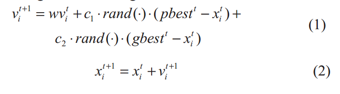
式中, vit是迭代次数为t时粒子i的速度,xit是迭代次数为t时粒子i的位置。粒子的速度通常限制在区间[-vmax, vmax]内。c1和c2是学习因子;rand()是统一来自[0,1]的随机数。PBestt和GBestt分别是迭代次数为t时所有粒子的个体最佳位置和全局最佳位置。变量w是迭代次数为t时的惯性权重,其定义如下:
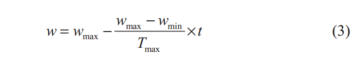
其中wmax和wmin分别是惯性重量的最大值和最小值,tmax是最大迭代次数。一般来说,wmax=0.9,wmin=0.4。
2.2BP神经网络
BP神经网络的结构是三层网络:输入层、隐藏层和输出层。在本文中,我们选择八个节点作为输入层。输出层中只有一个节点,即是是弹药储存可靠性预测值。由于隐层影响网络的鲁棒性,采用Hecht-Nelson方法[11]确定隐层的节点数。隐藏层h的节点数范围由三种公式确定:2n+1、√(n+m)+α和(m+n)/2,其中n是输入层的节点数,m是输出层的节点数,α是[1,10]中的常数。
3.PSO-BP神经网络预测方法
粒子群优化算法优化的BP神经网络即为是PSO-BP算法。文中提出的PSO-BP神经网络可用于弹药贮存可靠性的预测。PSO-BP算法优化了粒子群算法训练神经元的权值和偏差。PSO-BP算法的总体工作流程如图1所示
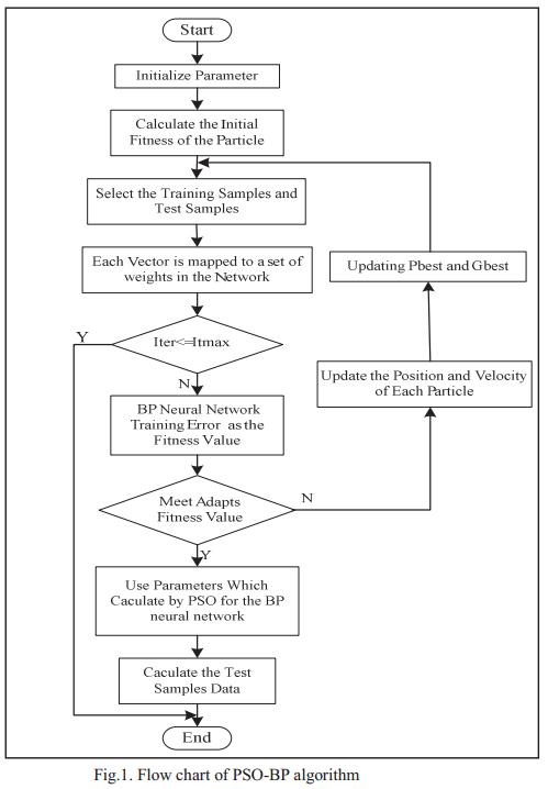
该算法的具体步骤描述如下:
step1:将训练数据集和测试数据集规范化为[0,1]之间。在标准化之后,为网络构建训练和测试样本。设置神经网络的输入层节点数、隐藏层节点数、输出层节点数。
step2:随机产生初始的一组种群规模为N 的粒子及其位置和速度。设置参数,例如迭代次数、惯性权重和学习因子。计算推断的网络输出向量和权重矩阵变化。
step3:计算每次迭代时每个粒子的适应度值,并记录全局极值和个体极值。更新每个粒子的位置和速度。将个体极值与全局极值进行比较。如果粒子个体极值优于全局最佳值,则更新全局最佳值。
step4:使用当前gbest值更新每个神经元的权值和偏值。选择MSE函数作为性能函数,用均方误差表示![]() 其中yid和yi分别是网络输出的期望值和实际值。
其中yid和yi分别是网络输出的期望值和实际值。
4.仿真实验的实现
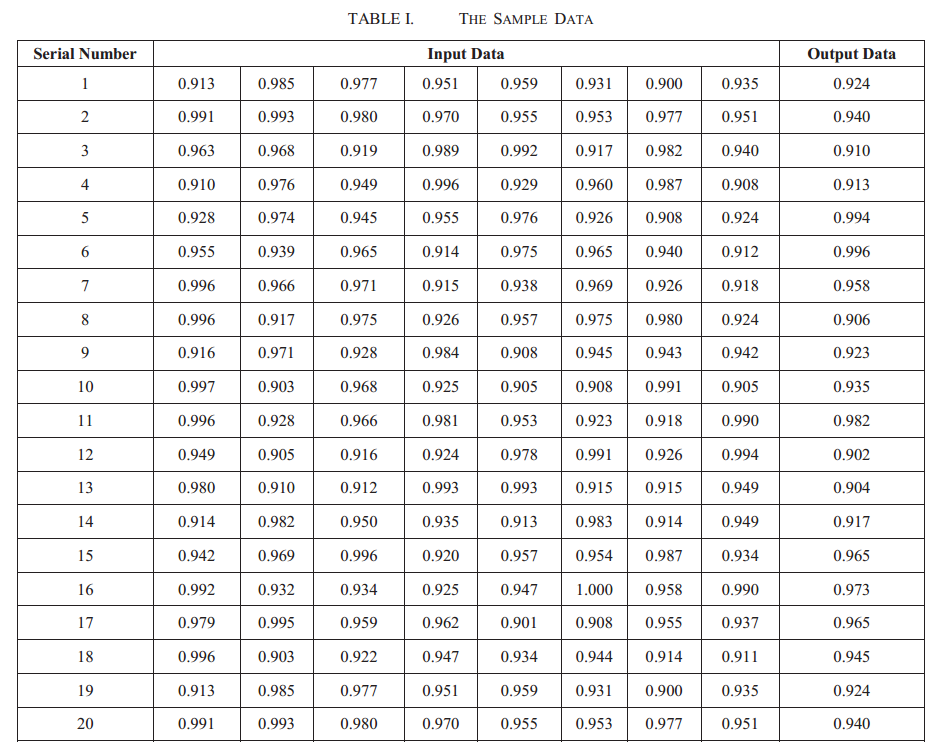
4.1数据集
论文中选取了20组弹药数据进行实验,如下图所示,其中前12组为训练集,后8组为测试集,每一组数组的前8列为输入,最后一列为输出,该数据是已经经过归一化处理后的数据。
4.2BP神经网络和PSO的参数设置
(1)BP神经网络的参数设置:
输入层节点:8
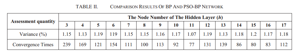
隐藏层节点:11(通过训练3-17的发现11是最优的)
输出层节点:1
最大训练次数:10000
学习率:0.5
精度:0.001
激活函数:tansig和logsig
训练函数:分别采用了traingdm和traingda进行对比
其中隐藏层是经过分别选取3-17的数作为隐藏层节点,然后训练网络,发现选择11的效果最好,如下图:
(2)PSO的参数设置:
粒子数目:30
维度:D=(n+m)*h+h+m n:输入层节点数,m:输出层节点数,h:隐藏层节点数
最大速度:1
学习因子:c1=c2=2
最大迭代次数:1000
惯性权重:wmax =0.9 , wmin =0.4.
4.3实验仿真结果
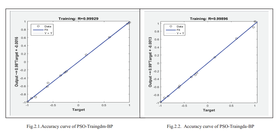

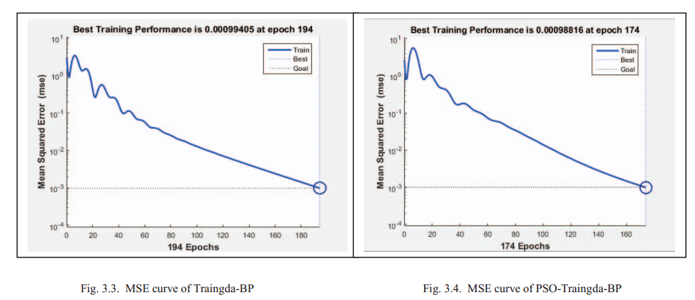
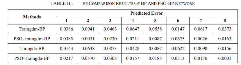
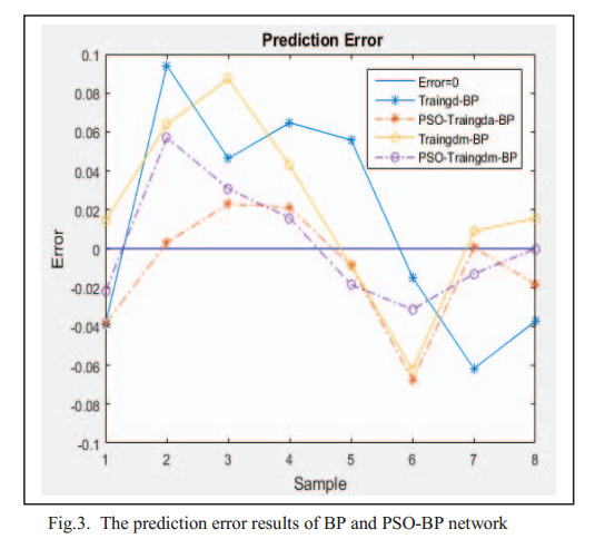
BP神经网络和PSOBP神经网络的实验结果如表3所示。可以看出,PSO-BP方法的性能优于BP方法。图2.1和图2.2表明,PSO-BP方法的预测精度大于98%。从图3.1—图3.4可以看出,当训练要求精度达到0.01时,两种算法都能满足预测误差的精度。PSO-BP方法的迭代次数小于BP方法的迭代次数。这意味着算法是收敛的。MSE曲线进一步说明了PSO-BP方法的稳定性优于BP方法。最后的图表明,PSO-BP方法的预测误差小于BP方法。结果表明,与常规BP算法相比,PSO-BP算法在最优参数搜索中具有更好的性能。PSO-BP方法的预测性能更适合于弹药储存的可靠性。
5.总结
文章运用了粒子群算法来优化BP神经网络中的权值和阈值,以此来提高弹药存储预测性能,而且预测精度也确实得到了提高,但由于数据集共有20组(也许是弹药数据的特殊性),还是觉得结果可能难以让人信服,但思路确实还是有用的,准备后面把该文的实验复现一下,或者用其他数据量比较大的预测数据,看下结果,再看一下有哪些还能值得改进的地方。

c# – Google Drive SDK System.Net.Http.Primitives版本1.5.0.0而不是2.1.10.0
<runtime>
<assemblybinding xmlns="urn:schemas-microsoft-com:asm.v1">
  <dependentassembly>
    <assemblyidentity name="System.Net.Http.Primitives"
                        culture="neutral"
                        publickeytoken="b03f5f7f11d50a3a"/>
    <bindingredirect newVersion="2.1.10.0" oldVersion="1.5.0.0"/>
  </dependentassembly>
</assemblybinding>
</runtime>
我只是缺少一些概念,还是有一个我需要下载的不同文件或者什么?
解决方法
今天的关于在ojAlgo中将两个矩阵或PrimitiveDenseStores进行元素相乘和两个矩阵元素对应相乘lingo的分享已经结束,谢谢您的关注,如果想了解更多关于An overview of gradient descent optimization algorithms、An universal algorithm design of fixed length substring locating、BP neural network optimized by PSO algorithm on Ammunition storage reliability prediction 阅读笔记、c# – Google Drive SDK System.Net.Http.Primitives版本1.5.0.0而不是2.1.10.0的相关知识,请在本站进行查询。
本文标签:


