本文的目的是介绍神经网络参数计算--直接解析CKPT文件读取的详细情况，特别关注神经网络checkpoint的相关信息。我们将通过专业的研究、有关数据的分析等多种方式，为您呈现一个全面的了解神经网络参

本文的目的是介绍神经网络 参数计算--直接解析CKPT文件读取的详细情况，特别关注神经网络checkpoint的相关信息。我们将通过专业的研究、有关数据的分析等多种方式，为您呈现一个全面的了解神经网络 参数计算--直接解析CKPT文件读取的机会，同时也不会遗漏关于01.神经网络和深度学习 W3.浅层神经网络（作业：带一个隐藏层的神经网络）、01.神经网络和深度学习 W4.深层神经网络（作业：建立你的深度神经网络+图片猫预测）、bp神经网络参数怎么设置,bp神经网络参数设置、CNN (卷积神经网络)、RNN (循环神经网络)、DNN (深度神经网络) 的内部网络结构有什么区别？的知识。

• 神经网络 参数计算--直接解析CKPT文件读取（神经网络checkpoint）
• 01.神经网络和深度学习 W3.浅层神经网络（作业：带一个隐藏层的神经网络）
• 01.神经网络和深度学习 W4.深层神经网络（作业：建立你的深度神经网络+图片猫预测）
• bp神经网络参数怎么设置,bp神经网络参数设置
• CNN (卷积神经网络)、RNN (循环神经网络)、DNN (深度神经网络) 的内部网络结构有什么区别？

神经网络 参数计算--直接解析CKPT文件读取（神经网络checkpoint）

1、tensorflow的模型文件ckpt参数获取

import tensoflow as tf
from tensorflow.python import pywrap_tensorflow
 
model_dir = "./ckpt/"
 
ckpt = tf.train.get_checkpoint_state(model_dir)
ckpt_path = ckpt.model_checkpoint_path
 
reader = pywrap_tensorflow.NewCheckpointReader(ckpt_path)
param_dict = reader.get_variable_to_shape_map()
 
for key, val in param_dict.items():
    try:
        print key, val
    except:

2、参数计算（求网络模型大小）

from tensorflow.python import pywrap_tensorflow
import os
import numpy as np
model_dir = "models_pretrained/"
checkpoint_path = os.path.join(model_dir, "model.ckpt-82798")
reader = pywrap_tensorflow.NewCheckpointReader(checkpoint_path)
var_to_shape_map = reader.get_variable_to_shape_map()
total_parameters = 0
for key in var_to_shape_map:#list the keys of the model
    # print(key)
    # print(reader.get_tensor(key))
    shape = np.shape(reader.get_tensor(key))  #get the shape of the tensor in the model
    shape = list(shape)
    # print(shape)
    # print(len(shape))
    variable_parameters = 1
    for dim in shape:
        # print(dim)
        variable_parameters *= dim
    # print(variable_parameters)
    total_parameters += variable_parameters

print(total_parameters)

01.神经网络和深度学习 W3.浅层神经网络（作业：带一个隐藏层的神经网络）

选择题测试：
参考博文1
参考博文2

建立你的第一个神经网络！其有1个隐藏层。

1. 导入包

# Package imports
import numpy as np
import matplotlib.pyplot as plt
from testCases import *
import sklearn
import sklearn.datasets
import sklearn.linear_model
from planar_utils import plot_decision_boundary, sigmoid, load_planar_dataset, load_extra_datasets

%matplotlib inline

np.random.seed(1) # set a seed so that the results are consistent

2. 预览数据

• 可视化数据

X, Y = load_planar_dataset()
# Visualize the data:
plt.scatter(X[0, :], X[1, :], c=Y, s=40, cmap=plt.cm.Spectral);

红色的标签为 0， 蓝色的标签为 1，我们的目标是建模将它们分开

• 数据维度

### START CODE HERE ### (≈ 3 lines of code)
shape_X = X.shape
shape_Y = Y.shape
m = X.shape[1]  # training set size
### END CODE HERE ###

print (''The shape of X is: '' + str(shape_X))
print (''The shape of Y is: '' + str(shape_Y))
print (''I have m = %d training examples!'' % (m))

The shape of X is: (2, 400)
The shape of Y is: (1, 400)
I have m = 400 training examples!

3. 逻辑回归

# Train the logistic regression classifier
clf = sklearn.linear_model.LogisticRegressionCV();
clf.fit(X.T, Y.T);

# Plot the decision boundary for logistic regression
plot_decision_boundary(lambda x: clf.predict(x), X, Y)
plt.title("Logistic Regression")

# Print accuracy
LR_predictions = clf.predict(X.T)
print (''Accuracy of logistic regression: %d '' % float((np.dot(Y,LR_predictions) + np.dot(1-Y,1-LR_predictions))/float(Y.size)*100) +
       ''% '' + "(percentage of correctly labelled datapoints)")

Accuracy of logistic regression: 47 % (percentage of correctly labelled datapoints)

数据集是线性不可分的，逻辑回归变现的不好，下面看看神经网络怎么样。

4. 神经网络

模型如下：

对于一个样本 x ( i ) x^{(i)} x(i) 而言：
z [ 1 ] ( i ) = W [ 1 ] x ( i ) + b [ 1 ] ( i ) z^{[1] (i)} = W^{[1]} x^{(i)} + b^{[1] (i)} z[1](i)=W[1]x(i)+b[1](i)
a [ 1 ] ( i ) = tanh ⁡ ( z [ 1 ] ( i ) ) a^{[1] (i)} = \tanh(z^{[1] (i)}) a[1](i)=tanh(z[1](i))
z [ 2 ] ( i ) = W [ 2 ] a [ 1 ] ( i ) + b [ 2 ] ( i ) z^{[2] (i)} = W^{[2]} a^{[1] (i)} + b^{[2] (i)} z[2](i)=W[2]a[1](i)+b[2](i)
y ^ ( i ) = a [ 2 ] ( i ) = σ ( z [ 2 ] ( i ) ) \hat{y}^{(i)} = a^{[2] (i)} = \sigma(z^{ [2] (i)}) y^​(i)=a[2](i)=σ(z[2](i))

y prediction ( i ) = { 1  if  a [ 2 ] ( i ) > 0.5 0  otherwise  y_{\text {prediction}}^{(i)}=\left\{\begin{array}{ll}1 & \text { if } a^{[2](i)}>0.5 \\ 0 & \text { otherwise }\end{array}\right. yprediction(i)​={10​ if a[2](i)>0.5 otherwise ​

得到所有的样本的预测值后，计算损失：
J = − 1 m ∑ i = 0 m ( y ( i ) log ⁡ ( a [ 2 ] ( i ) ) + ( 1 − y ( i ) ) log ⁡ ( 1 − a [ 2 ] ( i ) ) ) J = - \frac{1}{m} \sum\limits_{i = 0}^{m} \large\left(\small y^{(i)}\log\left(a^{[2] (i)}\right) + (1-y^{(i)})\log\left(1- a^{[2] (i)}\right) \large \right) \small J=−m1​i=0∑m​(y(i)log(a[2](i))+(1−y(i))log(1−a[2](i)))

建立神经网络的一般方法：

• 1、定义神经网络结构（输入，隐藏单元等）
• 2、初始化模型的参数
• 3、循环：
  —— a、实现正向传播
  —— b、计算损失
  —— c、实现反向传播，计算梯度
  —— d、更新参数（梯度下降）
  
  
  
  

编写辅助函数，计算步骤1-3
将它们合并到 nn_model（）的函数中
学习正确的参数，对新数据进行预测

4.1 定义神经网络结构

• 定义每层的节点个数

# GRADED FUNCTION: layer_sizes

def layer_sizes(X, Y):
    """
    Arguments:
    X -- input dataset of shape (input size, number of examples)
    Y -- labels of shape (output size, number of examples)
    
    Returns:
    n_x -- the size of the input layer
    n_h -- the size of the hidden layer
    n_y -- the size of the output layer
    """
    ### START CODE HERE ### (≈ 3 lines of code)
    n_x = X.shape[0] # size of input layer
    n_h = 4
    n_y = Y.shape[0] # size of output layer
    ### END CODE HERE ###
    return (n_x, n_h, n_y)

4.2 初始化模型参数

• 随机初始化权重 w，偏置 b 初始化为 0

# GRADED FUNCTION: initialize_parameters

def initialize_parameters(n_x, n_h, n_y):
    """
    Argument:
    n_x -- size of the input layer
    n_h -- size of the hidden layer
    n_y -- size of the output layer
    
    Returns:
    params -- python dictionary containing your parameters:
                    W1 -- weight matrix of shape (n_h, n_x)
                    b1 -- bias vector of shape (n_h, 1)
                    W2 -- weight matrix of shape (n_y, n_h)
                    b2 -- bias vector of shape (n_y, 1)
    """
    
    np.random.seed(2) # we set up a seed so that your output matches ours although the initialization is random.
    
    ### START CODE HERE ### (≈ 4 lines of code)
    W1 = np.random.randn(n_h, n_x)*0.01 # randn 标准正态分布
    b1 = np.zeros((n_h, 1))
    W2 = np.random.randn(n_y, n_h)*0.01
    b2 = np.zeros((n_y, 1))
    ### END CODE HERE ###
    
    assert (W1.shape == (n_h, n_x))
    assert (b1.shape == (n_h, 1))
    assert (W2.shape == (n_y, n_h))
    assert (b2.shape == (n_y, 1))
    
    parameters = {"W1": W1,
                  "b1": b1,
                  "W2": W2,
                  "b2": b2}
    
    return parameters

4.3 循环

4.3.1 前向传播

• 根据上面的公式，编写代码

# GRADED FUNCTION: forward_propagation

def forward_propagation(X, parameters):
    """
    Argument:
    X -- input data of size (n_x, m)
    parameters -- python dictionary containing your parameters 
    (output of initialization function)
    
    Returns:
    A2 -- The sigmoid output of the second activation
    cache -- a dictionary containing "Z1", "A1", "Z2" and "A2"
    """
    # Retrieve each parameter from the dictionary "parameters"
    ### START CODE HERE ### (≈ 4 lines of code)
    W1 = parameters[''W1'']
    b1 = parameters[''b1'']
    W2 = parameters[''W2'']
    b2 = parameters[''b2'']
    ### END CODE HERE ###
    
    # Implement Forward Propagation to calculate A2 (probabilities)
    ### START CODE HERE ### (≈ 4 lines of code)
    Z1 = np.dot(W1, X) + b1
    A1 = np.tanh(Z1)
    Z2 = np.dot(W2, A1) + b2
    A2 = sigmoid(Z2)
    ### END CODE HERE ###
    
    assert(A2.shape == (1, X.shape[1]))
    
    cache = {"Z1": Z1,
             "A1": A1,
             "Z2": Z2,
             "A2": A2}
    
    return A2, cache

4.3.2 计算损失

• 计算了 A2，也就是每个样本的预测值，计算损失
  J = − 1 m ∑ i = 0 m ( y ( i ) log ⁡ ( a [ 2 ] ( i ) ) + ( 1 − y ( i ) ) log ⁡ ( 1 − a [ 2 ] ( i ) ) ) J = - \frac{1}{m} \sum\limits_{i = 0}^{m} \large\left(\small y^{(i)}\log\left(a^{[2] (i)}\right) + (1-y^{(i)})\log\left(1- a^{[2] (i)}\right) \large \right) \small J=−m1​i=0∑m​(y(i)log(a[2](i))+(1−y(i))log(1−a[2](i)))
  

# GRADED FUNCTION: compute_cost

def compute_cost(A2, Y, parameters):
    """
    Computes the cross-entropy cost given in equation (13)
    
    Arguments:
    A2 -- The sigmoid output of the second activation, of shape (1, number of examples)
    Y -- "true" labels vector of shape (1, number of examples)
    parameters -- python dictionary containing your parameters W1, b1, W2 and b2
    
    Returns:
    cost -- cross-entropy cost given equation (13)
    """
    
    m = Y.shape[1] # number of example

    # Compute the cross-entropy cost
    ### START CODE HERE ### (≈ 2 lines of code)
    logprobs = Y*np.log(A2)+(1-Y)*np.log(1-A2)
    cost = -np.sum(logprobs)/m
    ### END CODE HERE ###
    
    cost = np.squeeze(cost)     # makes sure cost is the dimension we expect. 
                                # E.g., turns [[17]] into 17 
    assert(isinstance(cost, float))
    
    return cost

4.3.3 后向传播

一些公式如下：

激活函数的导数，请查阅

• sigmoid
  
  a = g ( z ) ; g ′ ( z ) = d d z g ( z ) = a ( 1 − a ) a=g(z) ;\quad g^{\prime}(z)=\frac{d}{d z} g(z)=a(1-a) a=g(z);g′(z)=dzd​g(z)=a(1−a)
  
  
• tanh
  
  a = g ( z ) ; g ′ ( z ) = d d z g ( z ) = 1 − a 2 a=g(z) ; \quad g^{\prime}(z)=\frac{d}{d z} g(z)=1-a^2 a=g(z);g′(z)=dzd​g(z)=1−a2
  
  

sigmoid 下损失函数求导

# GRADED FUNCTION: backward_propagation

def backward_propagation(parameters, cache, X, Y):
    """
    Implement the backward propagation using the instructions above.
    
    Arguments:
    parameters -- python dictionary containing our parameters 
    cache -- a dictionary containing "Z1", "A1", "Z2" and "A2".
    X -- input data of shape (2, number of examples)
    Y -- "true" labels vector of shape (1, number of examples)
    
    Returns:
    grads -- python dictionary containing your gradients with respect to different parameters
    """
    m = X.shape[1]
    
    # First, retrieve W1 and W2 from the dictionary "parameters".
    ### START CODE HERE ### (≈ 2 lines of code)
    W1 = parameters[''W1'']
    W2 = parameters[''W2'']
    ### END CODE HERE ###
        
    # Retrieve also A1 and A2 from dictionary "cache".
    ### START CODE HERE ### (≈ 2 lines of code)
    A1 = cache[''A1'']
    A2 = cache[''A2'']
    ### END CODE HERE ###
    
    # Backward propagation: calculate dW1, db1, dW2, db2. 
    ### START CODE HERE ### (≈ 6 lines of code, corresponding to 6 equations on slide above)
    dZ2 = A2-Y
    dW2 = np.dot(dZ2, A1.T)/m
    db2 = np.sum(dZ2, axis=1, keepdims=True)/m
    dZ1 = np.dot(W2.T, dZ2)*(1-np.power(A1, 2))
    dW1 = np.dot(dZ1, X.T)/m
    db1 = np.sum(dZ1, axis=1, keepdims=True)/m
    ### END CODE HERE ###
    
    grads = {"dW1": dW1,
             "db1": db1,
             "dW2": dW2,
             "db2": db2}
    
    return grads

4.3.4 梯度下降

• 选取合适的学习率，学习率太大，会产生震荡，收敛慢，甚至不收敛

# GRADED FUNCTION: update_parameters

def update_parameters(parameters, grads, learning_rate = 1.2):
    """
    Updates parameters using the gradient descent update rule given above
    
    Arguments:
    parameters -- python dictionary containing your parameters 
    grads -- python dictionary containing your gradients 
    
    Returns:
    parameters -- python dictionary containing your updated parameters 
    """
    # Retrieve each parameter from the dictionary "parameters"
    ### START CODE HERE ### (≈ 4 lines of code)
    W1 = parameters[''W1'']
    b1 = parameters[''b1'']
    W2 = parameters[''W2'']
    b2 = parameters[''b2'']
    ### END CODE HERE ###
    
    # Retrieve each gradient from the dictionary "grads"
    ### START CODE HERE ### (≈ 4 lines of code)
    dW1 = grads[''dW1'']
    db1 = grads[''db1'']
    dW2 = grads[''dW2'']
    db2 = grads[''db2'']
    ## END CODE HERE ###
    
    # Update rule for each parameter
    ### START CODE HERE ### (≈ 4 lines of code)
    W1 = W1 - learning_rate * dW1
    b1 = b1 - learning_rate * db1
    W2 = W2 - learning_rate * dW2
    b2 = b2 - learning_rate * db2
    ### END CODE HERE ###
    
    parameters = {"W1": W1,
                  "b1": b1,
                  "W2": W2,
                  "b2": b2}
    
    return parameters

4.4 组建Model

• 将上面的函数以正确顺序放在 model 里

# GRADED FUNCTION: nn_model

def nn_model(X, Y, n_h, num_iterations = 10000, print_cost=False):
    """
    Arguments:
    X -- dataset of shape (2, number of examples)
    Y -- labels of shape (1, number of examples)
    n_h -- size of the hidden layer
    num_iterations -- Number of iterations in gradient descent loop
    print_cost -- if True, print the cost every 1000 iterations
    
    Returns:
    parameters -- parameters learnt by the model. They can then be used to predict.
    """
    
    np.random.seed(3)
    n_x = layer_sizes(X, Y)[0]
    n_y = layer_sizes(X, Y)[2]
    
    # Initialize parameters, then retrieve W1, b1, W2, b2. Inputs: "n_x, n_h, n_y". 
    # Outputs = "W1, b1, W2, b2, parameters".
    ### START CODE HERE ### (≈ 5 lines of code)
    parameters = initialize_parameters(n_x, n_h, n_y)
    W1 = parameters[''W1'']
    b1 = parameters[''b1'']
    W2 = parameters[''W2'']
    b2 = parameters[''b2'']
    ### END CODE HERE ###
    
    # Loop (gradient descent)

    for i in range(0, num_iterations):
         
        ### START CODE HERE ### (≈ 4 lines of code)
        # Forward propagation. Inputs: "X, parameters". Outputs: "A2, cache".
        A2, cache = forward_propagation(X, parameters)
        
        # Cost function. Inputs: "A2, Y, parameters". Outputs: "cost".
        cost = compute_cost(A2, Y, parameters)
 
        # Backpropagation. Inputs: "parameters, cache, X, Y". Outputs: "grads".
        grads = backward_propagation(parameters, cache, X, Y)
 
        # Gradient descent parameter update. Inputs: "parameters, grads". Outputs: "parameters".
        parameters = update_parameters(parameters, grads, learning_rate=1.2)
        
        ### END CODE HERE ###
        
        # Print the cost every 1000 iterations
        if print_cost and i % 1000 == 0:
            print ("Cost after iteration %i: %f" %(i, cost))

    return parameters

4.5 预测

p r e d i c t i o n s = { 1 if  a c t i v a t i o n > 0.5 0 otherwise predictions = \begin{cases} 1 & \text{if}\ activation > 0.5 \\ 0 & \text{otherwise} \end{cases} predictions={10​if activation>0.5otherwise​

# GRADED FUNCTION: predict

def predict(parameters, X):
    """
    Using the learned parameters, predicts a class for each example in X
    
    Arguments:
    parameters -- python dictionary containing your parameters 
    X -- input data of size (n_x, m)
    
    Returns
    predictions -- vector of predictions of our model (red: 0 / blue: 1)
    """
    
    # Computes probabilities using forward propagation, and classifies to 0/1 using 0.5 as the threshold.
    ### START CODE HERE ### (≈ 2 lines of code)
    A2, cache = forward_propagation(X, parameters)
    predictions = (A2 > 0.5)
    ### END CODE HERE ###
    
    return predictions

• 建立一个含有1个隐藏层（4个单元）的神经网络模型

# Build a model with a n_h-dimensional hidden layer
parameters = nn_model(X, Y, n_h = 4, num_iterations = 10000, print_cost=True)

# Plot the decision boundary
plot_decision_boundary(lambda x: predict(parameters, x.T), X, Y)
plt.title("Decision Boundary for hidden layer size " + str(4))

Cost after iteration 0: 0.693048
Cost after iteration 1000: 0.288083
Cost after iteration 2000: 0.254385
Cost after iteration 3000: 0.233864
Cost after iteration 4000: 0.226792
Cost after iteration 5000: 0.222644
Cost after iteration 6000: 0.219731
Cost after iteration 7000: 0.217504
Cost after iteration 8000: 0.219550
Cost after iteration 9000: 0.218633

# Print accuracy
predictions = predict(parameters, X)
print (''Accuracy: %d'' % float((np.dot(Y,predictions.T) + np.dot(1-Y,1-predictions.T))/float(Y.size)*100) + ''%'')

Accuracy: 90%

可以看出模型较好地将两类点分开了！准确率 90%，比逻辑回归 47%高不少。

4.6 调节隐藏层单元个数

plt.figure(figsize=(16, 32))
hidden_layer_sizes = [1, 2, 3, 4, 5, 20, 50]
for i, n_h in enumerate(hidden_layer_sizes):
    plt.subplot(5, 2, i+1)
    plt.title(''Hidden Layer of size %d'' % n_h)
    parameters = nn_model(X, Y, n_h, num_iterations = 5000)
    plot_decision_boundary(lambda x: predict(parameters, x.T), X, Y)
    predictions = predict(parameters, X)
    accuracy = float((np.dot(Y,predictions.T) + np.dot(1-Y,1-predictions.T))/float(Y.size)*100)
    print ("Accuracy for {} hidden units: {} %".format(n_h, accuracy))

Accuracy for 1 hidden units: 67.5 %
Accuracy for 2 hidden units: 67.25 %
Accuracy for 3 hidden units: 90.75 %
Accuracy for 4 hidden units: 90.5 %
Accuracy for 5 hidden units: 91.25 %
Accuracy for 20 hidden units: 90.5 %
Accuracy for 50 hidden units: 90.75 %

可以看出：

• 较大的模型（具有更多隐藏单元）能够更好地适应训练集，直到最大的模型过拟合了
• 最好的隐藏层大小似乎是n_h=5左右。这个值似乎很适合数据，而不会引起明显的过拟合
• 稍后还将了解正则化，它允许你使用非常大的模型（如n_h=50），而不会出现太多过拟合

4.7 更改激活函数

• 将隐藏层的激活函数更改为 sigmoid 函数，准确率没有使用tanh的高，tanh在任何场合几乎都优于sigmoid

Accuracy for 1 hidden units: 50.5 %
Accuracy for 2 hidden units: 59.0 %
Accuracy for 3 hidden units: 56.75 %
Accuracy for 4 hidden units: 50.0 %
Accuracy for 5 hidden units: 62.25000000000001 %
Accuracy for 20 hidden units: 85.5 %
Accuracy for 50 hidden units: 87.0 %

• 将隐藏层的激活函数更改为 ReLu 函数，似乎没有用，感觉是需要更多的隐藏层，才能达到效果

def relu(X):
    return np.maximum(0, X)

Accuracy for 1 hidden units: 50.0 %
Accuracy for 2 hidden units: 50.0 %
Accuracy for 3 hidden units: 50.0 %
Accuracy for 4 hidden units: 50.0 %
Accuracy for 5 hidden units: 50.0 %
Accuracy for 20 hidden units: 50.0 %
Accuracy for 50 hidden units: 50.0 %

报了些警告

C:\Users\mingm\AppData\Roaming\Python\Python37\site-packages\
ipykernel_launcher.py:20: RuntimeWarning: divide by zero encountered in log
C:\Users\mingm\AppData\Roaming\Python\Python37\site-packages\
ipykernel_launcher.py:20: RuntimeWarning: invalid value encountered in multiply
C:\Users\mingm\AppData\Roaming\Python\Python37\site-packages\
ipykernel_launcher.py:35: RuntimeWarning: overflow encountered in power
C:\Users\mingm\AppData\Roaming\Python\Python37\site-packages\
ipykernel_launcher.py:35: RuntimeWarning: invalid value encountered in multiply
C:\Users\mingm\AppData\Roaming\Python\Python37\site-packages
\ipykernel_launcher.py:35: RuntimeWarning: overflow encountered in multiply

4.8 更改学习率

• 采用 tanh 激活函数，调整学习率检查效果

学习率 2.0

Accuracy for 1 hidden units: 67.5 %
Accuracy for 2 hidden units: 67.25 %
Accuracy for 3 hidden units: 90.75 %
Accuracy for 4 hidden units: 90.75 %
Accuracy for 5 hidden units: 90.25 %
Accuracy for 20 hidden units: 91.0 %
Accuracy for 50 hidden units: 91.25 %  best

学习率 1.5

Accuracy for 1 hidden units: 67.5 %
Accuracy for 2 hidden units: 67.25 %
Accuracy for 3 hidden units: 90.75 %
Accuracy for 4 hidden units: 89.75 %
Accuracy for 5 hidden units: 90.5 %
Accuracy for 20 hidden units: 91.0 %  best
Accuracy for 50 hidden units: 90.75 %

学习率 1.2

Accuracy for 1 hidden units: 67.5 %
Accuracy for 2 hidden units: 67.25 %
Accuracy for 3 hidden units: 90.75 %
Accuracy for 4 hidden units: 90.5 %
Accuracy for 5 hidden units: 91.25 % best
Accuracy for 20 hidden units: 90.5 %
Accuracy for 50 hidden units: 90.75 %

学习率 1.0

Accuracy for 1 hidden units: 67.25 %
Accuracy for 2 hidden units: 67.0 %
Accuracy for 3 hidden units: 90.75 %
Accuracy for 4 hidden units: 90.5 %
Accuracy for 5 hidden units: 91.0 %  best
Accuracy for 20 hidden units: 91.0 %  best
Accuracy for 50 hidden units: 90.75 %

学习率 0.5

Accuracy for 1 hidden units: 67.25 %
Accuracy for 2 hidden units: 66.5 %
Accuracy for 3 hidden units: 89.25 %
Accuracy for 4 hidden units: 90.0 %
Accuracy for 5 hidden units: 89.75 %
Accuracy for 20 hidden units: 90.0 % best
Accuracy for 50 hidden units: 89.75 %

学习率 0.1

Accuracy for 1 hidden units: 67.0 %
Accuracy for 2 hidden units: 64.75 %
Accuracy for 3 hidden units: 88.25 %
Accuracy for 4 hidden units: 88.0 %
Accuracy for 5 hidden units: 88.5 %
Accuracy for 20 hidden units: 88.75 %  best
Accuracy for 50 hidden units: 88.75 %  best

大致规律：

• 学习率太小，造成学习不充分，准确率较低
• 学习率越大，需要越多的隐藏单元来提高准确率？（请大佬指点）

4.9 其他数据集下的表现

均为tanh激活函数，学习率1.2

• dataset = "noisy_circles"
  
  

Accuracy for 1 hidden units: 62.5 %
Accuracy for 2 hidden units: 72.5 %
Accuracy for 3 hidden units: 84.0 % best
Accuracy for 4 hidden units: 83.0 %
Accuracy for 5 hidden units: 83.5 %
Accuracy for 20 hidden units: 79.5 %
Accuracy for 50 hidden units: 83.5 %

• dataset = "noisy_moons"
  
  

Accuracy for 1 hidden units: 86.0 %
Accuracy for 2 hidden units: 88.0 %
Accuracy for 3 hidden units: 97.0 % best
Accuracy for 4 hidden units: 96.5 %
Accuracy for 5 hidden units: 96.0 %
Accuracy for 20 hidden units: 86.0 %
Accuracy for 50 hidden units: 86.0 %

• dataset = "blobs"
  
  

Accuracy for 1 hidden units: 67.0 %
Accuracy for 2 hidden units: 67.0 %
Accuracy for 3 hidden units: 83.0 %
Accuracy for 4 hidden units: 83.0 %
Accuracy for 5 hidden units: 83.0 %
Accuracy for 20 hidden units: 86.0 % best
Accuracy for 50 hidden units: 83.5 %

• dataset = "gaussian_quantiles"
  
  

Accuracy for 1 hidden units: 65.0 %
Accuracy for 2 hidden units: 79.5 %
Accuracy for 3 hidden units: 97.0 %
Accuracy for 4 hidden units: 97.0 %
Accuracy for 5 hidden units: 100.0 % best
Accuracy for 20 hidden units: 97.5 %
Accuracy for 50 hidden units: 96.0 %

不同的数据集下，表现的效果也太一样。

我的CSDN博客地址 https://michael.blog.csdn.net/

长按或扫码关注我的公众号（Michael阿明），一起加油、一起学习进步！

01.神经网络和深度学习 W4.深层神经网络（作业：建立你的深度神经网络+图片猫预测）

测试题：参考博文

作业1. 建立你的深度神经网络

1. 导入包

import numpy as np
import h5py
import matplotlib.pyplot as plt
from testCases_v2 import *
from dnn_utils_v2 import sigmoid, sigmoid_backward, relu, relu_backward

%matplotlib inline
plt.rcParams[''figure.figsize''] = (5.0, 4.0) # set default size of plots
plt.rcParams[''image.interpolation''] = ''nearest''
plt.rcParams[''image.cmap''] = ''gray''

%load_ext autoreload
%autoreload 2

np.random.seed(1)

2. 算法主要流程

3. 初始化

第4节笔记：01.神经网络和深度学习 W4.深层神经网络

3.1 两层神经网络

模型结构：LINEAR -> RELU -> LINEAR -> SIGMOID
权重：np.random.randn(shape)*0.01
偏置：np.zeros(shape)

# GRADED FUNCTION: initialize_parameters

def initialize_parameters(n_x, n_h, n_y):
    """
    Argument:
    n_x -- size of the input layer
    n_h -- size of the hidden layer
    n_y -- size of the output layer
    
    Returns:
    parameters -- python dictionary containing your parameters:
                    W1 -- weight matrix of shape (n_h, n_x)
                    b1 -- bias vector of shape (n_h, 1)
                    W2 -- weight matrix of shape (n_y, n_h)
                    b2 -- bias vector of shape (n_y, 1)
    """
    
    np.random.seed(1)
    
    ### START CODE HERE ### (≈ 4 lines of code)
    W1 = np.random.randn(n_h, n_x)*0.01
    b1 = np.zeros((n_h, 1))
    W2 = np.random.randn(n_y, n_h)*0.01
    b2 = np.zeros((n_y, 1))
    ### END CODE HERE ###
    
    assert(W1.shape == (n_h, n_x))
    assert(b1.shape == (n_h, 1))
    assert(W2.shape == (n_y, n_h))
    assert(b2.shape == (n_y, 1))
    
    parameters = {"W1": W1,
                  "b1": b1,
                  "W2": W2,
                  "b2": b2}
    
    return parameters    

3.2 多层神经网络

模型结构：[LINEAR -> RELU] × (L-1) -> LINEAR -> SIGMOID

# GRADED FUNCTION: initialize_parameters_deep

def initialize_parameters_deep(layer_dims):
    """
    Arguments:
    layer_dims -- python array (list) containing the dimensions of each layer in our network
    
    Returns:
    parameters -- python dictionary containing your parameters "W1", "b1", ..., "WL", "bL":
                    Wl -- weight matrix of shape (layer_dims[l], layer_dims[l-1])
                    bl -- bias vector of shape (layer_dims[l], 1)
    """
    
    np.random.seed(3)
    parameters = {}
    L = len(layer_dims)            # number of layers in the network

    for l in range(1, L):
        ### START CODE HERE ### (≈ 2 lines of code)
        parameters[''W'' + str(l)] = np.random.randn(layer_dims[l], layer_dims[l-1])*0.01
        parameters[''b'' + str(l)] = np.zeros((layer_dims[l], 1))
        ### END CODE HERE ###
        
        assert(parameters[''W'' + str(l)].shape == (layer_dims[l], layer_dims[l-1]))
        assert(parameters[''b'' + str(l)].shape == (layer_dims[l], 1))

        
    return parameters

4. 前向传播

4.1 线性模块

向量化公式
Z [ l ] = W [ l ] A [ l − 1 ] + b [ l ] Z^{[l]} = W^{[l]}A^{[l-1]} +b^{[l]} Z[l]=W[l]A[l−1]+b[l]

其中 A [ 0 ] = X A^{[0]} = X A[0]=X

计算 Z Z Z，缓存 A , W , b A, W, b A,W,b

# GRADED FUNCTION: linear_forward

def linear_forward(A, W, b):
    """
    Implement the linear part of a layer''s forward propagation.

    Arguments:
    A -- activations from previous layer (or input data): 
        (size of previous layer, number of examples)
    W -- weights matrix: numpy array of shape 
        (size of current layer, size of previous layer)
    b -- bias vector, numpy array of shape 
        (size of the current layer, 1)

    Returns:
    Z -- the input of the activation function, 
        also called pre-activation parameter 
    cache -- a python dictionary containing "A", "W" and "b" ; 
    stored for computing the backward pass efficiently
    """
    
    ### START CODE HERE ### (≈ 1 line of code)
    Z = np.dot(W, A) + b
    ### END CODE HERE ###
    
    assert(Z.shape == (W.shape[0], A.shape[1]))
    cache = (A, W, b)
    
    return Z, cache

4.2 线性激活模块

计算激活输出 A A A，以及缓存 Z Z Z （反向传播时要用到）（作业里的激活函数会返回这两项）
A [ l ] = g ( Z [ l ] ) = g ( W [ l ] A [ l − 1 ] + b [ l ] ) A^{[l]} = g(Z^{[l]}) = g(W^{[l]}A^{[l-1]} +b^{[l]}) A[l]=g(Z[l])=g(W[l]A[l−1]+b[l])
其中 g g g 是激活函数，可以是ReLu，Sigmoid等

# GRADED FUNCTION: linear_activation_forward

def linear_activation_forward(A_prev, W, b, activation):
    """
    Implement the forward propagation for the LINEAR->ACTIVATION layer

    Arguments:
    A_prev -- activations from previous layer (or input data): 
        (size of previous layer, number of examples)
    W -- weights matrix: numpy array of shape 
        (size of current layer, size of previous layer)
    b -- bias vector, numpy array of shape 
        (size of the current layer, 1)
    activation -- the activation to be used in this layer, 
        stored as a text string: "sigmoid" or "relu"

    Returns:
    A -- the output of the activation function, 
        also called the post-activation value 
    cache -- a python dictionary containing "linear_cache" and "activation_cache";
             stored for computing the backward pass efficiently
    """
    
    if activation == "sigmoid":
        # Inputs: "A_prev, W, b". Outputs: "A, activation_cache".
        ### START CODE HERE ### (≈ 2 lines of code)
        Z, linear_cache = linear_forward(A_prev, W, b)
        A, activation_cache = sigmoid(Z)
        ### END CODE HERE ###
    
    elif activation == "relu":
        # Inputs: "A_prev, W, b". Outputs: "A, activation_cache".
        ### START CODE HERE ### (≈ 2 lines of code)
        Z, linear_cache = linear_forward(A_prev, W, b)
        A, activation_cache = relu(Z)
        ### END CODE HERE ###
    
    assert (A.shape == (W.shape[0], A_prev.shape[1]))
    cache = (linear_cache, activation_cache)

    return A, cache

4.3 多层模型

前面使用 L − 1 L-1 L−1 层 ReLu，最后使用 1 层 Sigmoid

# GRADED FUNCTION: L_model_forward

def L_model_forward(X, parameters):
    """
    Implement forward propagation for the 
        [LINEAR->RELU]*(L-1)->LINEAR->SIGMOID computation
    
    Arguments:
    X -- data, numpy array of shape 
        (input size, number of examples)
    parameters -- output of initialize_parameters_deep()
    
    Returns:
    AL -- last post-activation value
    caches -- list of caches containing:
                every cache of linear_relu_forward() 
                    (there are L-1 of them, indexed from 0 to L-2)
                the cache of linear_sigmoid_forward() 
                    (there is one, indexed L-1)
    """

    caches = []
    A = X
    L = len(parameters) // 2   # number of layers in the neural network
    
    # Implement [LINEAR -> RELU]*(L-1). Add "cache" to the "caches" list.
    for l in range(1, L):
        A_prev = A 
        ### START CODE HERE ### (≈ 2 lines of code)
        A, cache = linear_activation_forward(A_prev, parameters[''W''+str(l)], parameters[''b''+str(l)], ''relu'')
        caches.append(cache) # 每一层的 （A，W，b, Z)
        ### END CODE HERE ###
    
    # Implement LINEAR -> SIGMOID. Add "cache" to the "caches" list.
    ### START CODE HERE ### (≈ 2 lines of code)
    AL, cache = linear_activation_forward(A, parameters[''W''+str(L)], parameters[''b''+str(L)], ''sigmoid'')
    caches.append(cache)
    ### END CODE HERE ###
    
    assert(AL.shape == (1,X.shape[1]))
            
    return AL, caches

现在得到了一个完整的前向传播，AL 包含预测值，可以计算损失函数

5. 损失函数

计算损失：

− 1 m ∑ i = 1 m ( y ( i ) log ⁡ ( a [ L ] ( i ) ) + ( 1 − y ( i ) ) log ⁡ ( 1 − a [ L ] ( i ) ) ) -\frac{1}{m} \sum\limits_{i = 1}^{m} \bigg(y^{(i)}\log\left(a^{[L] (i)}\right) + (1-y^{(i)})\log\left(1- a^{[L](i)}\right) \bigg) −m1​i=1∑m​(y(i)log(a[L](i))+(1−y(i))log(1−a[L](i)))

# GRADED FUNCTION: compute_cost

def compute_cost(AL, Y):
    """
    Implement the cost function defined by equation (7).

    Arguments:
    AL -- probability vector corresponding to your label predictions, shape (1, number of examples)
    Y -- true "label" vector (for example: containing 0 if non-cat, 1 if cat), shape (1, number of examples)

    Returns:
    cost -- cross-entropy cost
    """
    
    m = Y.shape[1]

    # Compute loss from aL and y.
    ### START CODE HERE ### (≈ 1 lines of code)
    cost = np.sum(Y*np.log(AL)+(1-Y)*np.log(1-AL))/(-m)
    ### END CODE HERE ###
    
    cost = np.squeeze(cost)      # To make sure your cost''s shape is what we expect (e.g. this turns [[17]] into 17).
    assert(cost.shape == ())
    
    return cost

6. 反向传播

计算损失函数的梯度：

6.1 线性模块

d W [ l ] = ∂ L ∂ W [ l ] = 1 m d Z [ l ] A [ l − 1 ] T dW^{[l]} = \frac{\partial \mathcal{L} }{\partial W^{[l]}} = \frac{1}{m} dZ^{[l]} A^{[l-1] T} dW[l]=∂W[l]∂L​=m1​dZ[l]A[l−1]T
d b [ l ] = ∂ L ∂ b [ l ] = 1 m ∑ i = 1 m d Z [ l ] ( i ) db^{[l]} = \frac{\partial \mathcal{L} }{\partial b^{[l]}} = \frac{1}{m} \sum_{i = 1}^{m} dZ^{[l](i)} db[l]=∂b[l]∂L​=m1​i=1∑m​dZ[l](i)
d A [ l − 1 ] = ∂ L ∂ A [ l − 1 ] = W [ l ] T d Z [ l ] dA^{[l-1]} = \frac{\partial \mathcal{L} }{\partial A^{[l-1]}} = W^{[l] T} dZ^{[l]} dA[l−1]=∂A[l−1]∂L​=W[l]TdZ[l]

# GRADED FUNCTION: linear_backward

def linear_backward(dZ, cache):
    """
    Implement the linear portion of backward propagation for a single layer (layer l)

    Arguments:
    dZ -- Gradient of the cost with respect to the linear output (of current layer l)
    cache -- tuple of values (A_prev, W, b) coming from the forward propagation in the current layer

    Returns:
    dA_prev -- Gradient of the cost with respect to the activation (of the previous layer l-1), same shape as A_prev
    dW -- Gradient of the cost with respect to W (current layer l), same shape as W
    db -- Gradient of the cost with respect to b (current layer l), same shape as b
    """
    A_prev, W, b = cache
    m = A_prev.shape[1]

    ### START CODE HERE ### (≈ 3 lines of code)
    dW = np.dot(dZ, A_prev.T)/m
    db = 1/m*np.sum(dZ, axis=1, keepdims=True)
    dA_prev = np.dot(W.T, dZ)
    ### END CODE HERE ###
    
    assert (dA_prev.shape == A_prev.shape)
    assert (dW.shape == W.shape)
    assert (db.shape == b.shape)
    
    return dA_prev, dW, db

6.2 线性激活模块

d Z [ l ] = d A [ l ] ∗ g ′ ( Z [ l ] ) dZ^{[l]} = dA^{[l]} * g''(Z^{[l]}) dZ[l]=dA[l]∗g′(Z[l])

# GRADED FUNCTION: linear_activation_backward

def linear_activation_backward(dA, cache, activation):
    """
    Implement the backward propagation for the LINEAR->ACTIVATION layer.
    
    Arguments:
    dA -- post-activation gradient for current layer l 
    cache -- tuple of values (linear_cache, activation_cache) we store for computing backward propagation efficiently
    activation -- the activation to be used in this layer, stored as a text string: "sigmoid" or "relu"
    
    Returns:
    dA_prev -- Gradient of the cost with respect to the activation (of the previous layer l-1), same shape as A_prev
    dW -- Gradient of the cost with respect to W (current layer l), same shape as W
    db -- Gradient of the cost with respect to b (current layer l), same shape as b
    """
    linear_cache, activation_cache = cache
    
    if activation == "relu":
        ### START CODE HERE ### (≈ 2 lines of code)
        dZ = relu_backward(dA, activation_cache)
        dA_prev, dW, db = linear_backward(dZ, linear_cache)
        ### END CODE HERE ###
        
    elif activation == "sigmoid":
        ### START CODE HERE ### (≈ 2 lines of code)
        dZ = sigmoid_backward(dA, activation_cache)
        dA_prev, dW, db = linear_backward(dZ, linear_cache)
        ### END CODE HERE ###
    
    return dA_prev, dW, db

6.3 多层模型

d A L = − n p . d i v i d e ( Y , A L ) + n p . d i v i d e ( 1 − Y , 1 − A L ) dAL = - np.divide(Y, AL) + np.divide(1 - Y, 1 - AL) dAL=−np.divide(Y,AL)+np.divide(1−Y,1−AL)

# GRADED FUNCTION: L_model_backward

def L_model_backward(AL, Y, caches):
    """
    Implement the backward propagation for the [LINEAR->RELU] * (L-1) -> LINEAR -> SIGMOID group
    
    Arguments:
    AL -- probability vector, output of the forward propagation (L_model_forward())
    Y -- true "label" vector (containing 0 if non-cat, 1 if cat)
    caches -- list of caches containing:
                every cache of linear_activation_forward() with "relu" 
                    (it''s caches[l], for l in range(L-1) i.e l = 0...L-2)
                the cache of linear_activation_forward() with "sigmoid" 
                    (it''s caches[L-1])
    
    Returns:
    grads -- A dictionary with the gradients
             grads["dA" + str(l)] = ... 
             grads["dW" + str(l)] = ...
             grads["db" + str(l)] = ... 
    """
    grads = {}
    L = len(caches) # the number of layers
    m = AL.shape[1]
    Y = Y.reshape(AL.shape) # after this line, Y is the same shape as AL
    
    # Initializing the backpropagation
    ### START CODE HERE ### (1 line of code)
    dAL = -np.divide(Y, AL) + np.divide(1-Y, 1-AL)
    ### END CODE HERE ###
    
    # Lth layer (SIGMOID -> LINEAR) gradients. 
    # Inputs: "AL, Y, caches". 
    # Outputs: "grads["dAL"], grads["dWL"], grads["dbL"]
    ### START CODE HERE ### (approx. 2 lines)
    current_cache = caches[L-1]
    grads["dA" + str(L)], grads["dW" + str(L)], grads["db" + str(L)] = linear_activation_backward(dAL, current_cache, ''sigmoid'')
    ### END CODE HERE ###
    
    for l in reversed(range(L-1)):
        # lth layer: (RELU -> LINEAR) gradients.
        # Inputs: "grads["dA" + str(l + 2)], caches". 
        # Outputs: "grads["dA" + str(l + 1)] , grads["dW" + str(l + 1)] , grads["db" + str(l + 1)] 
        ### START CODE HERE ### (approx. 5 lines)
        current_cache = caches[l]
        dA_prev_temp, dW_temp, db_temp = linear_activation_backward(grads[''dA''+str(l+2)], current_cache, ''relu'')
        grads["dA" + str(l + 1)] = dA_prev_temp
        grads["dW" + str(l + 1)] = dW_temp
        grads["db" + str(l + 1)] = db_temp
        ### END CODE HERE ###

    return grads

6.4 梯度下降、更新参数

W [ l ] = W [ l ] − α   d W [ l ] W^{[l]} = W^{[l]} - \alpha \text{ } dW^{[l]} W[l]=W[l]−α dW[l]
b [ l ] = b [ l ] − α   d b [ l ] b^{[l]} = b^{[l]} - \alpha \text{ } db^{[l]} b[l]=b[l]−α db[l]

# GRADED FUNCTION: update_parameters

def update_parameters(parameters, grads, learning_rate):
    """
    Update parameters using gradient descent
    
    Arguments:
    parameters -- python dictionary containing your parameters 
    grads -- python dictionary containing your gradients, output of L_model_backward
    
    Returns:
    parameters -- python dictionary containing your updated parameters 
                  parameters["W" + str(l)] = ... 
                  parameters["b" + str(l)] = ...
    """
    
    L = len(parameters) // 2 # number of layers in the neural network

    # Update rule for each parameter. Use a for loop.
    ### START CODE HERE ### (≈ 3 lines of code)
    for l in range(L):
        parameters["W" + str(l+1)] = parameters[''W''+str(l+1)] - learning_rate * grads[''dW''+str(l+1)]
        parameters["b" + str(l+1)] = parameters[''b''+str(l+1)] - learning_rate * grads[''db''+str(l+1)]
    ### END CODE HERE ###
        
    return parameters

作业2. 深度神经网络应用：图像分类

使用上面的函数，建立深度神经网络，并对图片是不是猫进行预测。

1. 导入包

import time
import numpy as np
import h5py
import matplotlib.pyplot as plt
import scipy
from PIL import Image
from scipy import ndimage
from dnn_app_utils_v2 import *

%matplotlib inline
plt.rcParams[''figure.figsize''] = (5.0, 4.0) # set default size of plots
plt.rcParams[''image.interpolation''] = ''nearest''
plt.rcParams[''image.cmap''] = ''gray''

%load_ext autoreload
%autoreload 2

np.random.seed(1)

2. 数据集

01.神经网络和深度学习 W2.神经网络基础（作业：逻辑回归 图片识别）

使用 01W2 作业里面的数据集，逻辑回归的准确率只有 70%

• 加载数据

train_x_orig, train_y, test_x_orig, test_y, classes = load_data()

• 查看数据

# Example of a picture
index = 1
plt.imshow(train_x_orig[index])
print ("y = " + str(train_y[0,index]) + ". It''s a " + classes[train_y[0,index]].decode("utf-8") +  " picture.")

• 查看数据大小

# Explore your dataset 
m_train = train_x_orig.shape[0]
num_px = train_x_orig.shape[1]
m_test = test_x_orig.shape[0]

print ("Number of training examples: " + str(m_train))
print ("Number of testing examples: " + str(m_test))
print ("Each image is of size: (" + str(num_px) + ", " + str(num_px) + ", 3)")
print ("train_x_orig shape: " + str(train_x_orig.shape))
print ("train_y shape: " + str(train_y.shape))
print ("test_x_orig shape: " + str(test_x_orig.shape))
print ("test_y shape: " + str(test_y.shape))

Number of training examples: 209
Number of testing examples: 50
Each image is of size: (64, 64, 3)
train_x_orig shape: (209, 64, 64, 3)
train_y shape: (1, 209)
test_x_orig shape: (50, 64, 64, 3)
test_y shape: (1, 50)

• 图片数据向量化
  
  

# Reshape the training and test examples 
train_x_flatten = train_x_orig.reshape(train_x_orig.shape[0], -1).T   # The "-1" makes reshape flatten the remaining dimensions
test_x_flatten = test_x_orig.reshape(test_x_orig.shape[0], -1).T

# Standardize data to have feature values between 0 and 1.
train_x = train_x_flatten/255.
test_x = test_x_flatten/255.

print ("train_x''s shape: " + str(train_x.shape))
print ("test_x''s shape: " + str(test_x.shape))

train_x''s shape: (12288, 209) # 12288 = 64 * 64 * 3
test_x''s shape: (12288, 50)

3. 建立模型

3.1 两层神经网络

3.2 多层神经网络

3.3 一般步骤

1. 初始化参数 / 定义超参数
2. n_iters次 迭代循环：
   – a. 正向传播
   – b. 计算成本函数
   – c. 反向传播
   – d. 更新参数（使用参数、梯度）
   
   
   
   
3. 使用训练好的参数 预测

4. 两层神经网络

• 定义参数

### CONSTANTS DEFINING THE MODEL ####
n_x = 12288     # num_px * num_px * 3
n_h = 7  # 隐藏层单元个数
n_y = 1
layers_dims = (n_x, n_h, n_y)

• 组件模型

# GRADED FUNCTION: two_layer_model

def two_layer_model(X, Y, layers_dims, learning_rate = 0.0075, num_iterations = 3000, print_cost=False):
    """
    Implements a two-layer neural network: LINEAR->RELU->LINEAR->SIGMOID.
    
    Arguments:
    X -- input data, of shape (n_x, number of examples)
    Y -- true "label" vector (containing 0 if cat, 1 if non-cat), of shape (1, number of examples)
    layers_dims -- dimensions of the layers (n_x, n_h, n_y)
    num_iterations -- number of iterations of the optimization loop
    learning_rate -- learning rate of the gradient descent update rule
    print_cost -- If set to True, this will print the cost every 100 iterations 
    
    Returns:
    parameters -- a dictionary containing W1, W2, b1, and b2
    """
    
    np.random.seed(1)
    grads = {}
    costs = []                              # to keep track of the cost
    m = X.shape[1]                           # number of examples
    (n_x, n_h, n_y) = layers_dims
    
    # Initialize parameters dictionary, by calling one of the functions you''d previously implemented
    ### START CODE HERE ### (≈ 1 line of code)
    parameters = initialize_parameters(n_x, n_h, n_y)
    ### END CODE HERE ###
    
    # Get W1, b1, W2 and b2 from the dictionary parameters.
    W1 = parameters["W1"]
    b1 = parameters["b1"]
    W2 = parameters["W2"]
    b2 = parameters["b2"]
    
    # Loop (gradient descent)

    for i in range(0, num_iterations):

        # Forward propagation: LINEAR -> RELU -> LINEAR -> SIGMOID. 
        # Inputs: "X, W1, b1". 
        # Output: "A1, cache1, A2, cache2".
        ### START CODE HERE ### (≈ 2 lines of code)
        A1, cache1 = linear_activation_forward(X, W1, b1, ''relu'')
        A2, cache2 = linear_activation_forward(A1, W2, b2, ''sigmoid'')
        ### END CODE HERE ###
        
        # Compute cost
        ### START CODE HERE ### (≈ 1 line of code)
        cost = compute_cost(A2, Y)
        ### END CODE HERE ###
        
        # Initializing backward propagation
        dA2 = - np.divide(Y, A2) + np.divide(1 - Y, 1 - A2)
        
        # Backward propagation. 
        # Inputs: "dA2, cache2, cache1". 
        # Outputs: "dA1, dW2, db2; also dA0 (not used), dW1, db1".
        ### START CODE HERE ### (≈ 2 lines of code)
        dA1, dW2, db2 = linear_activation_backward(dA2, cache2, ''sigmoid'')
        dA0, dW1, db1 = linear_activation_backward(dA1, cache1, ''relu'')
        ### END CODE HERE ###
        
        # Set grads[''dWl''] to dW1, grads[''db1''] to db1, grads[''dW2''] to dW2, grads[''db2''] to db2
        grads[''dW1''] = dW1
        grads[''db1''] = db1
        grads[''dW2''] = dW2
        grads[''db2''] = db2
        
        # Update parameters.
        ### START CODE HERE ### (approx. 1 line of code)
        parameters = update_parameters(parameters, grads, learning_rate)
        ### END CODE HERE ###

        # Retrieve W1, b1, W2, b2 from parameters
        W1 = parameters["W1"]
        b1 = parameters["b1"]
        W2 = parameters["W2"]
        b2 = parameters["b2"]
        
        # Print the cost every 100 training example
        if print_cost and i % 100 == 0:
            print("Cost after iteration {}: {}".format(i, np.squeeze(cost)))
        if print_cost and i % 100 == 0:
            costs.append(cost)
       
    # plot the cost

    plt.plot(np.squeeze(costs))
    plt.ylabel(''cost'')
    plt.xlabel(''iterations (per tens)'')
    plt.title("Learning rate =" + str(learning_rate))
    plt.show()
    
    return parameters

• 训练

parameters = two_layer_model(train_x, train_y, layers_dims = (n_x, n_h, n_y), num_iterations = 2500, print_cost=True)

Cost after iteration 0: 0.693049735659989
Cost after iteration 100: 0.6464320953428849
Cost after iteration 200: 0.6325140647912678
Cost after iteration 300: 0.6015024920354665
Cost after iteration 400: 0.5601966311605747
Cost after iteration 500: 0.5158304772764729
Cost after iteration 600: 0.4754901313943325
Cost after iteration 700: 0.43391631512257495
Cost after iteration 800: 0.4007977536203887
Cost after iteration 900: 0.35807050113237976
Cost after iteration 1000: 0.33942815383664127
Cost after iteration 1100: 0.30527536361962654
Cost after iteration 1200: 0.2749137728213016
Cost after iteration 1300: 0.24681768210614846
Cost after iteration 1400: 0.19850735037466097
Cost after iteration 1500: 0.17448318112556657
Cost after iteration 1600: 0.1708076297809689
Cost after iteration 1700: 0.11306524562164715
Cost after iteration 1800: 0.09629426845937145
Cost after iteration 1900: 0.08342617959726863
Cost after iteration 2000: 0.07439078704319078
Cost after iteration 2100: 0.06630748132267933
Cost after iteration 2200: 0.0591932950103817
Cost after iteration 2300: 0.05336140348560554
Cost after iteration 2400: 0.04855478562877016

• 预测

训练集：Accuracy: 0.9999999999999998

predictions_train = predict(train_x, train_y, parameters)
# Accuracy: 0.9999999999999998

测试集：Accuracy: 0.72，比之前的逻辑回归 0.70 好一些

predictions_test = predict(test_x, test_y, parameters)
# Accuracy: 0.72

5. 多层神经网络

• 定义参数，5层 NN

### CONSTANTS ###
layers_dims = [12288, 20, 7, 5, 1] #  5-layer model

• 组件模型

# GRADED FUNCTION: L_layer_model

def L_layer_model(X, Y, layers_dims, learning_rate = 0.0075, num_iterations = 3000, print_cost=False):#lr was 0.009
    """
    Implements a L-layer neural network: [LINEAR->RELU]*(L-1)->LINEAR->SIGMOID.
    
    Arguments:
    X -- data, numpy array of shape (number of examples, num_px * num_px * 3)
    Y -- true "label" vector (containing 0 if cat, 1 if non-cat), of shape (1, number of examples)
    layers_dims -- list containing the input size and each layer size, of length (number of layers + 1).
    learning_rate -- learning rate of the gradient descent update rule
    num_iterations -- number of iterations of the optimization loop
    print_cost -- if True, it prints the cost every 100 steps
    
    Returns:
    parameters -- parameters learnt by the model. They can then be used to predict.
    """

    np.random.seed(1)
    costs = []                         # keep track of cost
    
    # Parameters initialization.
    ### START CODE HERE ###
    parameters = initialize_parameters_deep(layers_dims)
    ### END CODE HERE ###
    
    # Loop (gradient descent)
    for i in range(0, num_iterations):

        # Forward propagation: [LINEAR -> RELU]*(L-1) -> LINEAR -> SIGMOID.
        ### START CODE HERE ### (≈ 1 line of code)
        AL, caches = L_model_forward(X, parameters)
        ### END CODE HERE ###
        
        # Compute cost.
        ### START CODE HERE ### (≈ 1 line of code)
        cost = compute_cost(AL, Y)
        ### END CODE HERE ###
    
        # Backward propagation.
        ### START CODE HERE ### (≈ 1 line of code)
        grads = L_model_backward(AL, Y, caches)
        ### END CODE HERE ###
 
        # Update parameters.
        ### START CODE HERE ### (≈ 1 line of code)
        parameters = update_parameters(parameters, grads, learning_rate)
        ### END CODE HERE ###
                
        # Print the cost every 100 training example
        if print_cost and i % 100 == 0:
            print ("Cost after iteration %i: %f" %(i, cost))
        if print_cost and i % 100 == 0:
            costs.append(cost)
            
    # plot the cost
    plt.plot(np.squeeze(costs))
    plt.ylabel(''cost'')
    plt.xlabel(''iterations (per tens)'')
    plt.title("Learning rate =" + str(learning_rate))
    plt.show()
    
    return parameters

• 训练

parameters = L_layer_model(train_x, train_y, layers_dims, num_iterations = 2500, print_cost = True)

Cost after iteration 0: 0.771749
Cost after iteration 100: 0.672053
Cost after iteration 200: 0.648263
Cost after iteration 300: 0.611507
Cost after iteration 400: 0.567047
Cost after iteration 500: 0.540138
Cost after iteration 600: 0.527930
Cost after iteration 700: 0.465477
Cost after iteration 800: 0.369126
Cost after iteration 900: 0.391747
Cost after iteration 1000: 0.315187
Cost after iteration 1100: 0.272700
Cost after iteration 1200: 0.237419
Cost after iteration 1300: 0.199601
Cost after iteration 1400: 0.189263
Cost after iteration 1500: 0.161189
Cost after iteration 1600: 0.148214
Cost after iteration 1700: 0.137775
Cost after iteration 1800: 0.129740
Cost after iteration 1900: 0.121225
Cost after iteration 2000: 0.113821
Cost after iteration 2100: 0.107839
Cost after iteration 2200: 0.102855
Cost after iteration 2300: 0.100897
Cost after iteration 2400: 0.092878

• 预测

训练集：Accuracy: 0.9856459330143539

pred_train = predict(train_x, train_y, parameters)
# Accuracy: 0.9856459330143539

测试集：Accuracy: 0.8，比逻辑回归 0.70，两层NN 0.72 都要好

pred_test = predict(test_x, test_y, parameters)
# Accuracy: 0.8

下一门课将会系统的学习如何调参，使得模型的效果更好

6. 结果分析

def print_mislabeled_images(classes, X, y, p):
    """
    Plots images where predictions and truth were different.
    X -- dataset
    y -- true labels
    p -- predictions
    """
    a = p + y
    mislabeled_indices = np.asarray(np.where(a == 1)) # 0+1, 1+0, wrong case
    plt.rcParams[''figure.figsize''] = (40.0, 40.0) # set default size of plots
    num_images = len(mislabeled_indices[0])
    for i in range(num_images):
        index = mislabeled_indices[1][i]
        
        plt.subplot(2, num_images, i + 1)
        plt.imshow(X[:,index].reshape(64,64,3), interpolation=''nearest'')
        plt.axis(''off'')
        plt.title("Prediction: " + classes[int(p[0,index])].decode("utf-8") + " \n Class: " + classes[y[0,index]].decode("utf-8"))

print_mislabeled_images(classes, test_x, test_y, pred_test)

错误特点：

• 猫的身体在一个不寻常的位置
• 猫出现在一个相似颜色的背景下
• 不常见的猫颜色和种类
• 照相机角度
• 图片的亮度
• 大小程度（猫在图像中非常大或很小）

7. 用自己的图片测试

## START CODE HERE ##
my_image = "my_image.jpg" # change this to the name of your image file 
my_label_y = [1] # the true class of your image (1 -> cat, 0 -> non-cat)
## END CODE HERE ##

fname = "images/" + my_image
image = Image.open(fname)
my_image = np.array(image.resize((num_px,num_px))).reshape((num_px*num_px*3,1))
my_predicted_image = predict(my_image, my_label_y, parameters)

plt.imshow(image)
print ("y = " + str(np.squeeze(my_predicted_image)) + ", your L-layer model predicts a \"" + classes[int(np.squeeze(my_predicted_image)),].decode("utf-8") +  "\" picture.")

Accuracy: 1.0
y = 1.0, your L-layer model predicts a "cat" picture.

我的CSDN博客地址 https://michael.blog.csdn.net/

长按或扫码关注我的公众号（Michael阿明），一起加油、一起学习进步！

bp神经网络参数怎么设置,bp神经网络参数设置

BP神经网络模型各个参数的选取问题

样本变量不需要那么多，因为神经网络的信息存储能力有限，过多的样本会造成一些有用的信息被丢弃。如果样本数量过多，应增加隐层节点数或隐层数目，才能增强学习能力。

一、隐层数一般认为，增加隐层数可以降低网络误差（也有文献认为不一定能有效降低），提高精度，但也使网络复杂化，从而增加了网络的训练时间和出现“过拟合”的倾向。

一般来讲应设计神经网络应优先考虑3层网络（即有1个隐层）。一般地，靠增加隐层节点数来获得较低的误差，其训练效果要比增加隐层数更容易实现。

对于没有隐层的神经网络模型，实际上就是一个线性或非线性（取决于输出层采用线性或非线性转换函数型式）回归模型。

因此，一般认为，应将不含隐层的网络模型归入回归分析中，技术已很成熟，没有必要在神经网络理论中再讨论之。

二、隐层节点数在BP网络中，隐层节点数的选择非常重要，它不仅对建立的神经网络模型的性能影响很大，而且是训练时出现“过拟合”的直接原因，但是目前理论上还没有一种科学的和普遍的确定方法。

目前多数文献中提出的确定隐层节点数的计算公式都是针对训练样本任意多的情况，而且多数是针对最不利的情况，一般工程实践中很难满足，不宜采用。事实上，各种计算公式得到的隐层节点数有时相差几倍甚至上百倍。

为尽可能避免训练时出现“过拟合”现象，保证足够高的网络性能和泛化能力，确定隐层节点数的最基本原则是：在满足精度要求的前提下取尽可能紧凑的结构，即取尽可能少的隐层节点数。

研究表明，隐层节点数不仅与输入/输出层的节点数有关，更与需解决的问题的复杂程度和转换函数的型式以及样本数据的特性等因素有关。

谷歌人工智能写作项目：爱发猫

BP神经网络中的训练函数如何选取

神经网络不同的网络有这不同的训练函数，BP神经网络有两种训练函数，trainbp（），利用BP算法训练前向神经网络AI爱发猫。

trainbpx（），利用快速BP算法训练前向神经网络，即采用了动量或自适应学习，可减少训练时间，tansig函数是神经元的传递函数，与训练函数无关，在trainbp（）函数中含有要训练神经元的函数。

matlab BP神经网络出错 newff参数 隐含层 怎么确定

。

设[P,T]是训练样本，[X,Y]是测试样本；net=newrb(P,T,err_goal,spread);%建立网络q=sim(net,p);e=q-T;plot(p,q);%画训练误差曲线q=sim(net,X);e=q-Y;plot(X,q);%画测试误差曲线训练前馈网络的第一步是建立网络对象。

函数newff建立一个可训练的前馈网络。这需要4个输入参数。第一个参数是一个Rx2的矩阵以定义R个输入向量的最小值和最大值。第二个参数是一个设定每层神经元个数的数组。

第三个参数是包含每层用到的传递函数名称的细胞数组。最后一个参数是用到的训练函数的名称。举个例子，下面命令将创建一个二层网络。

它的输入是两个元素的向量，第一层有三个神经元(3)，第二层有一个神经元(1)。第一层的传递函数是tan-sigmoid，输出层的传递函数是linear。

输入向量的第一个元素的范围是-1到2[-12]，输入向量的第二个元素的范围是0到5[05]，训练函数是traingd。

net=newff([-12;05],[3,1],{'tansig','purelin'},'traingd');这个命令建立了网络对象并且初始化了网络权重和偏置，因此网络就可以进行训练了。

我们可能要多次重新初始化权重或者进行自定义的初始化。下面就是初始化的详细步骤。在训练前馈网络之前，权重和偏置必须被初始化。初始化权重和偏置的工作用命令init来实现。

这个函数接收网络对象并初始化权重和偏置后返回网络对象。

下面就是网络如何初始化的：net=init(net);我们可以通过设定网络参数net.initFcn和net.layer{i}.initFcn这一技巧来初始化一个给定的网络。

net.initFcn用来决定整个网络的初始化函数。前馈网络的缺省值为initlay，它允许每一层用单独的初始化函数。

设定了net.initFcn，那么参数net.layer{i}.initFcn也要设定用来决定每一层的初始化函数。对前馈网络来说，有两种不同的初始化方式经常被用到：initwb和initnw。

initwb函数根据每一层自己的初始化参数(net.inputWeights{i,j}.initFcn)初始化权重矩阵和偏置。前馈网络的初始化权重通常设为rands，它使权重在-1到1之间随机取值。

这种方式经常用在转换函数是线性函数时。initnw通常用于转换函数是曲线函数。

它根据Nguyen和Widrow[NgWi90]为层产生初始权重和偏置值，使得每层神经元的活动区域能大致平坦的分布在输入空间。

BP神经网络中初始权值和阈值的设定

1、首先需要了解BP神经网络是一种多层前馈网络。2、以看一下在matlab中BP神经网络的训练函数，有梯度下降法traingd,弹性梯度下降法trainrp，自适应lr梯度下降法traingda等。

3、在matlab中命令行窗口中定义输入P，输出T，·通过“newff(minmax(P),[5,1]构建BP神经网络，“[net,tr]=train(net,P,T);”进行网络训练，“sim(net,P)”得到仿真预测值。

4、在命令行窗口按回车键之后，可以看到出现结果弹窗，最上面的NeuralNetwork下面依次代表的是“输入、隐含层、输出层、输出”，隐含层中有5个神经元。

5、Progress下面的Epoch代表迭代次数，Gradient代表梯度，VaildationChecks代表有效性检查，最后的绿色对勾代表性能目标达成。

6、最后将实际曲线和预测曲线绘制出来，可以看到使用BP神经网络预测的结果曲线基本和实际输出曲线一致。

BP网络中的trainlm训练函数，需要设置的参数？

。

以输出层权值更新的算法做说明：新w(i,j)=旧w(i,j)+a*E(i)O(j)+b*oldw(i,j),其中，新w(i,j)为计算一步以后的权，旧w(i,j)为初始权，E(i)为输出层第i个神经元的输出误差，O(j)为隐含层第j个神经元的输出数据，a学习系数，b惯性系数。

其实b就是优化设计中梯度下降法的步长，训练函数和梯度下降法是一个样子的，都是通过初始点，选定负梯度方向，计算步长，然后得到下一点，如此循环，神经网络把梯度下降法简化了，直接选定步长，不再计算步长了，

MATLAB中如何获取BP神经网络训练后的参数

sim命令将运行指定的模型。模型执行时使用传递给sim命令的数据，这些数据包括在options结构中设定的参数值。

a=sim(net,[])中，net是你的训练网络，后面的中括号是你要训练的结构参数！

BP神经网络输入层和训练次数怎样选择

CNN (卷积神经网络)、RNN (循环神经网络)、DNN (深度神经网络) 的内部网络结构有什么区别？

科言君

每周六提供一份高质量回答。

首先，我感觉不必像 @李 Shawn 同学一样认为 DNN、CNN、RNN 完全不能相提并论。从广义上来说，NN（或是更美的 DNN）确实可以认为包含了 CNN、RNN 这些具体的变种形式。在实际应用中，所谓的深度神经网络 DNN，往往融合了多种已知的结构，包括卷积层或是 LSTM 单元。但是就题主的意思来看，这里的 DNN 应该特指全连接的神经元结构，并不包含卷积单元或是时间上的关联。因此，题主一定要将 DNN、CNN、RNN 等进行对比，也未尝不可。

其实，如果我们顺着神经网络技术发展的脉络，就很容易弄清这几种网络结构发明的初衷，和他们之间本质的区别，希望对题主有所帮助。

=========================== 分 割 线 就 是 我 ================================

神经网络技术起源于上世纪五、六十年代，当时叫感知机（perceptron），拥有输入层、输出层和一个隐含层。输入的特征向量通过隐含层变换达到输出层，在输出层得到分类结果。早期感知机的推动者是 Rosenblatt。（扯一个不相关的：由于计算技术的落后，当时感知器传输函数是用线拉动变阻器改变电阻的方法机械实现的，脑补一下科学家们扯着密密麻麻的导线的样子…）

但是，Rosenblatt 的单层感知机有一个严重得不能再严重的问题，即它对稍复杂一些的函数都无能为力（比如最为典型的 “异或” 操作）。连异或都不能拟合，你还能指望这货有什么实际用途么 o (╯□╰) o

随着数学的发展，这个缺点直到上世纪八十年代才被 Rumelhart、Williams、Hinton、LeCun 等人（反正就是一票大牛）发明的多层感知机（multilayer perceptron）克服。多层感知机，顾名思义，就是有多个隐含层的感知机（废话……）。好好，我们看一下多层感知机的结构：

图 1 上下层神经元全部相连的神经网络 —— 多层感知机

多层感知机可以摆脱早期离散传输函数的束缚，使用 sigmoid 或 tanh 等连续函数模拟神经元对激励的响应，在训练算法上则使用 Werbos 发明的反向传播 BP 算法。对，这货就是我们现在所说的神经网络 NN—— 神经网络听起来不知道比感知机高端到哪里去了！这再次告诉我们起一个好听的名字对于研（zhuang）究（bi）很重要！

多层感知机解决了之前无法模拟异或逻辑的缺陷，同时更多的层数也让网络更能够刻画现实世界中的复杂情形。相信年轻如 Hinton 当时一定是春风得意。

多层感知机给我们带来的启示是，神经网络的层数直接决定了它对现实的刻画能力 —— 利用每层更少的神经元拟合更加复杂的函数 [1]。

（Bengio 如是说：functions that can be compactly represented by a depth k architecture might require an exponential number of computational elements to be represented by a depth k − 1 architecture.）

即便大牛们早就预料到神经网络需要变得更深，但是有一个梦魇总是萦绕左右。随着神经网络层数的加深，优化函数越来越容易陷入局部最优解，并且这个 “陷阱” 越来越偏离真正的全局最优。利用有限数据训练的深层网络，性能还不如较浅层网络。同时，另一个不可忽略的问题是随着网络层数增加，“梯度消失” 现象更加严重。具体来说，我们常常使用 sigmoid 作为神经元的输入输出函数。对于幅度为 1 的信号，在 BP 反向传播梯度时，每传递一层，梯度衰减为原来的 0.25。层数一多，梯度指数衰减后低层基本上接受不到有效的训练信号。

2006 年，Hinton 利用预训练方法缓解了局部最优解问题，将隐含层推动到了 7 层 [2]，神经网络真正意义上有了 “深度”，由此揭开了深度学习的热潮。这里的 “深度” 并没有固定的定义 —— 在语音识别中 4 层网络就能够被认为是 “较深的”，而在图像识别中 20 层以上的网络屡见不鲜。为了克服梯度消失，ReLU、maxout 等传输函数代替了 sigmoid，形成了如今 DNN 的基本形式。单从结构上来说，全连接的 DNN 和图 1 的多层感知机是没有任何区别的。

值得一提的是，今年出现的高速公路网络（highway network）和深度残差学习（deep residual learning）进一步避免了梯度消失，网络层数达到了前所未有的一百多层（深度残差学习：152 层）[3,4]！具体结构题主可自行搜索了解。如果你之前在怀疑是不是有很多方法打上了 “深度学习” 的噱头，这个结果真是深得让人心服口服。

图 2 缩减版的深度残差学习网络，仅有 34 层，终极版有 152 层，自行感受一下

如图 1 所示，我们看到全连接 DNN 的结构里下层神经元和所有上层神经元都能够形成连接，带来的潜在问题是参数数量的膨胀。假设输入的是一幅像素为 1K*1K 的图像，隐含层有 1M 个节点，光这一层就有 10^12 个权重需要训练，这不仅容易过拟合，而且极容易陷入局部最优。另外，图像中有固有的局部模式（比如轮廓、边界，人的眼睛、鼻子、嘴等）可以利用，显然应该将图像处理中的概念和神经网络技术相结合。此时我们可以祭出题主所说的卷积神经网络 CNN。对于 CNN 来说，并不是所有上下层神经元都能直接相连，而是通过 “卷积核” 作为中介。同一个卷积核在所有图像内是共享的，图像通过卷积操作后仍然保留原先的位置关系。两层之间的卷积传输的示意图如下：

图 3 卷积神经网络隐含层（摘自 Theano 教程）

通过一个例子简单说明卷积神经网络的结构。假设图 3 中 m-1=1 是输入层，我们需要识别一幅彩色图像，这幅图像具有四个通道 ARGB（透明度和红绿蓝，对应了四幅相同大小的图像），假设卷积核大小为 100*100，共使用 100 个卷积核 w1 到 w100（从直觉来看，每个卷积核应该学习到不同的结构特征）。用 w1 在 ARGB 图像上进行卷积操作，可以得到隐含层的第一幅图像；这幅隐含层图像左上角第一个像素是四幅输入图像左上角 100*100 区域内像素的加权求和，以此类推。同理，算上其他卷积核，隐含层对应 100 幅 “图像”。每幅图像对是对原始图像中不同特征的响应。按照这样的结构继续传递下去。CNN 中还有 max-pooling 等操作进一步提高鲁棒性。

图 4 一个典型的卷积神经网络结构，注意到最后一层实际上是一个全连接层（摘自 Theano 教程）

在这个例子里，我们注意到输入层到隐含层的参数瞬间降低到了 100*100*100=10^6 个！这使得我们能够用已有的训练数据得到良好的模型。题主所说的适用于图像识别，正是由于 CNN 模型限制参数了个数并挖掘了局部结构的这个特点。顺着同样的思路，利用语音语谱结构中的局部信息，CNN 照样能应用在语音识别中。

全连接的 DNN 还存在着另一个问题 —— 无法对时间序列上的变化进行建模。然而，样本出现的时间顺序对于自然语言处理、语音识别、手写体识别等应用非常重要。对了适应这种需求，就出现了题主所说的另一种神经网络结构 —— 循环神经网络 RNN。

在普通的全连接网络或 CNN 中，每层神经元的信号只能向上一层传播，样本的处理在各个时刻独立，因此又被成为前向神经网络 (Feed-forward Neural Networks)。而在 RNN 中，神经元的输出可以在下一个时间戳直接作用到自身，即第 i 层神经元在 m 时刻的输入，除了（i-1）层神经元在该时刻的输出外，还包括其自身在（m-1）时刻的输出！表示成图就是这样的：

图 5 RNN 网络结构

我们可以看到在隐含层节点之间增加了互连。为了分析方便，我们常将 RNN 在时间上进行展开，得到如图 6 所示的结构：

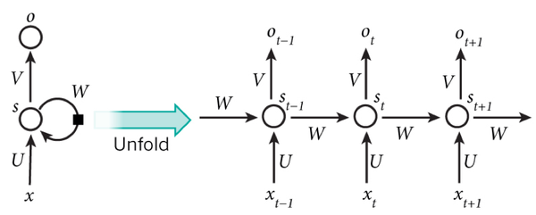
图 6 RNN 在时间上进行展开

Cool，（t+1）时刻网络的最终结果 O (t+1) 是该时刻输入和所有历史共同作用的结果！这就达到了对时间序列建模的目的。

不知题主是否发现，RNN 可以看成一个在时间上传递的神经网络，它的深度是时间的长度！正如我们上面所说，“梯度消失” 现象又要出现了，只不过这次发生在时间轴上。对于 t 时刻来说，它产生的梯度在时间轴上向历史传播几层之后就消失了，根本就无法影响太遥远的过去。因此，之前说 “所有历史” 共同作用只是理想的情况，在实际中，这种影响也就只能维持若干个时间戳。

为了解决时间上的梯度消失，机器学习领域发展出了长短时记忆单元 LSTM，通过门的开关实现时间上记忆功能，并防止梯度消失，一个 LSTM 单元长这个样子：

图 7 LSTM 的模样

除了题主疑惑的三种网络，和我之前提到的深度残差学习、LSTM 外，深度学习还有许多其他的结构。举个例子，RNN 既然能继承历史信息，是不是也能吸收点未来的信息呢？因为在序列信号分析中，如果我能预知未来，对识别一定也是有所帮助的。因此就有了双向 RNN、双向 LSTM，同时利用历史和未来的信息。

图 8 双向 RNN

事实上，不论是那种网络，他们在实际应用中常常都混合着使用，比如 CNN 和 RNN 在上层输出之前往往会接上全连接层，很难说某个网络到底属于哪个类别。不难想象随着深度学习热度的延续，更灵活的组合方式、更多的网络结构将被发展出来。尽管看起来千变万化，但研究者们的出发点肯定都是为了解决特定的问题。题主如果想进行这方面的研究，不妨仔细分析一下这些结构各自的特点以及它们达成目标的手段。入门的话可以参考：

Ng 写的 Ufldl：UFLDL 教程 - Ufldl

也可以看 Theano 内自带的教程，例子非常具体：Deep Learning Tutorials

欢迎大家继续推荐补充。

当然啦，如果题主只是想凑个热闹时髦一把，或者大概了解一下方便以后把妹使，这样看看也就罢了吧。

参考文献：

[1] Bengio Y. Learning Deep Architectures for AI[J]. Foundations & Trends® in Machine Learning, 2009, 2(1):1-127.

[2] Hinton G E, Salakhutdinov R R. Reducing the Dimensionality of Data with Neural Networks[J]. Science, 2006, 313(5786):504-507.

[3] He K, Zhang X, Ren S, Sun J. Deep Residual Learning for Image Recognition. arXiv:1512.03385, 2015.

[4] Srivastava R K, Greff K, Schmidhuber J. Highway networks. arXiv:1505.00387, 2015.

【“科研君” 公众号初衷始终是希望聚集各专业一线科研人员和工作者，在进行科学研究的同时也作为知识的传播者，利用自己的专业知识解释和普及生活中的 一些现象和原理，展现科学有趣生动的一面。该公众号由清华大学一群在校博士生发起，目前参与的作者人数有 10 人，但我们感觉这远远不能覆盖所以想科普的领域，并且由于空闲时间有限，导致我们只能每周发布一篇文章。我们期待更多的战友加入，认识更多志同道合的人，每个人都是科研君，每个人都是知识的传播者。我们期待大家的参与，想加入我们，进 QQ 群吧～：108141238】

 

【非常高兴看到大家喜欢并赞同我们的回答。应许多知友的建议，最近我们开通了同名公众号：PhDer，也会定期更新我们的文章，如果您不想错过我们的每篇回答，欢迎扫码关注～】

http://weixin.qq.com/r/5zsuNoHEZdwarcVV9271 (二维码自动识别)

编辑于 2016-07-19

李 Shawn

PhD candidate

个人觉得 CNN、RNN 和 DNN 不能放在一起比较。
DNN 是一个大类，CNN 是一个典型的空间上深度的神经网络，RNN 是在时间上深度的神经网络。
推荐你从 UFLDL 开始看，这是斯坦福深度学习的课程，了解一些神经网络的基础，会对你的学习有很大帮助。
============================= 分割线 ======================================
前面一位同学回答得非常详细完整，我再回来谈一谈怎么学习这些模型，我来分享一下我的学习历程。我也是在学习中，以后会慢慢继续补充。
1、http://ufldl.stanford.edu/wiki/index.php/UFLDL 教程
这是我最开始接触神经网络时看的资料，把这个仔细研究完会对神经网络的模型以及如何训练（反向传播算法）有一个基本的认识，算是一个基本功。

2、Deep Learning Tutorials
这是一个开源的深度学习工具包，里面有很多深度学习模型的 python 代码还有一些对模型以及代码细节的解释。我觉得学习深度学习光了解模型是不难的，难点在于把模型落地写成代码，因为里面会有很多细节只有动手写了代码才会了解。但 Theano 也有缺点，就是极其难以调试，以至于我后来就算自己动手写几百行的代码也不愿意再用它的工具包。所以我觉得 Theano 的正确用法还是在于看里面解释的文字，不要害怕英文，这是必经之路。PS：推荐使用 python 语言，目前来看比较主流。（更新：自己写坑实在太多了，CUDA 也不知道怎么用，还是乖乖用 theano 吧...）

3、Stanford University CS231n: Convolutional Neural Networks for Visual Recognition
斯坦福的一门课：卷积神经网络，李飞飞教授主讲。这门课会系统的讲一下卷积神经网络的模型，然后还有一些课后习题，题目很有代表性，也是用 python 写的，是在一份代码中填写一部分缺失的代码。如果把这个完整学完，相信使用卷积神经网络就不是一个大问题了。

4、斯坦福大学公开课 ：机器学习课程
这可能是机器学习领域最经典最知名的公开课了，由大牛 Andrew Ng 主讲，这个就不仅仅是深度学习了，它是带你领略机器学习领域中最重要的概念，然后建立起一个框架，使你对机器学习这个学科有一个较为完整的认识。这个我觉得所有学习机器学习的人都应该看一下，我甚至在某公司的招聘要求上看到过：认真看过并深入研究过 Andrew Ng 的机器学习课程，由此可见其重要性。

编辑于 2016-04-20

YJango

1

日本会津大学 人机界面实验室博士在读

2017 年 7 月 3 日 更新

不同网络的区别：人们在网络中实现加入的先验知识的不同。

整体解释：公开课 | 深层神经网络设计理念 附带 ppt 下载（无视频版）

神经网络入门：深层学习为何要 “Deep”（上）

前馈神经网络引入的先验知识：并行、迭代；

• 详细解释：深层学习为何要 “Deep”（下） 较难懂，建议先看完公开课再看该篇文章。

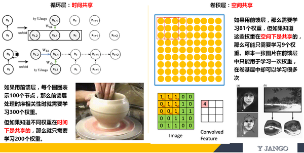
循环神经网络引入的先验知识：时间共享；

• 详细解释：循环神经网络 -- 介绍

循环神经网络引入的先验知识：空间共享；

• 详细解释：卷积神经网络 -- 介绍

深层学习的 “深” 字是由于将分类 / 回归和特征提取两者结合在一起来训练了。

Recurrent layer 和 convolutional layer 都可以看成是特征提取层。

1. 语音识别用 Recurrent layer 去学习 “如何” 去听，再用学好的听取方式去处理声音再送入分类器中。人脑举例子，我们大脑已有从中文学来的对语音的 “特征提取层” 和 “分类层”。学习外语的时候，只是新训练了一个 “分类层”，继续用中文的语音的 “特征提取层”，这是外语听力的不好的原因之一。
2. 画面识别 convolutional layer 学习 “如何” 去观察，再用学好的观察方式去处理画面再送入分类器中。人脑举例子，我们在观察图片的时候并不是一眼把所有画面都送入大脑进行识别的，而是跟 convolutional layer 的处理方式一样，逐一扫描局部后再合并。不同的扫描方式，所观察出的内容也不同。

具体可以看下面的部分

简单理解神经网络应该分为两部分：

• 网络结构：神经网络是怎么计算预测的，以及神经网络为什么好用。
• 网络训练：神经网络是怎么训练的，以及如何克服在训练时所遇到的如过拟合，梯度消失等问题。

进一步理解围绕 “深层” 二字来神经网络的的话应该在网络结构中细分两类： 网络结构：

• 特征结构：之所以要深层是因为一部分的层在完成 “学习如何提取特征” 的任务。比如画面处理的 convolutional layers ，时间序列处理的 Recurrent layers。甚至 feedforward layers 也能完成此任务。
• 分类 / 递归结构：如果仅需完成分类器的任务的话，一个 hidden feedforward 足以。其他的机器学习算法如 SVM，GP 甚至做的要比神经网络要好。

举例说明：比如图片识别。一个图片究竟是什么不仅取决于图片本身，还取决于识别者 “如何观察”。

如果这是一个训练样本。

• 当你给的标签是少女的时候，convolutional layers 会以此学习 “如何观察” 成少女
• 当你给的标签是老妇的时候，convolutional layers 会以此学习 “如何观察” 成老妇
• 之所以深层，是因为一定数量的层数在学习 “如何观察”。再学习完如何观察后再传递给 “分类层” 中去。而分类层并不需要 “深”。
• 网络结构中最重要的是特征结构层，画面处理的 convolutional layers ，时间序列处理的 Recurrent layers 最好理解为特征结构层。

编辑于 2017-07-11

许铁 - 巡洋舰科技

微信公众号请关注 chaoscruiser , 铁哥个人微信号 ironcruiser

首先， 要看 RNN 和对于图像等静态类变量处理立下神功的卷积网络 CNN 的结构区别来看， “循环” 两个字，已经点出了 RNN 的核心特征， 即系统的输出会保留在网络里， 和系统下一刻的输入一起共同决定下一刻的输出。这就把动力学的本质体现了出来， 循环正对应动力学系统的反馈概念，可以刻画复杂的历史依赖。另一个角度看也符合著名的图灵机原理。 即此刻的状态包含上一刻的历史，又是下一刻变化的依据。 这其实包含了可编程神经网络的核心概念，即， 当你有一个未知的过程，但你可以测量到输入和输出， 你假设当这个过程通过 RNN 的时候，它是可以自己学会这样的输入输出规律的， 而且因此具有预测能力。 在这点上说， RNN 是图灵完备的。

图： 图 1 即 CNN 的架构， 图 2 到 5 是 RNN 的几种基本玩法。图 2 是把单一输入转化为序列输出，例如把图像转化成一行文字。 图三是把序列输入转化为单个输出， 比如情感测试，测量一段话正面或负面的情绪。 图四是把序列转化为序列， 最典型的是机器翻译， 注意输入和输出的 “时差”。 图 5 是无时差的序列到序列转化， 比如给一个录像中的每一帧贴标签。 图片来源 The unreasonable effective RNN。

我们用一段小巧的 python 代码让你重新理解下上述的原理：

classRNN:

# ...

def step(self, x):

# update the hidden state

self.h = np.tanh(np.dot(self.W_hh, self.h) + np.dot(self.W_xh, x))

# compute the output vector

y = np.dot(self.W_hy, self.h)

return y

这里的 h 就是 hidden variable 隐变量，即整个网络每个神经元的状态，x 是输入， y 是输出， 注意着三者都是高维向量。隐变量 h，就是通常说的神经网络本体，也正是循环得以实现的基础， 因为它如同一个可以储存无穷历史信息 (理论上) 的水库，一方面会通过输入矩阵 W_xh 吸收输入序列 x 的当下值，一方面通过网络连接 W_hh 进行内部神经元间的相互作用（网络效应，信息传递），因为其网络的状态和输入的整个过去历史有关， 最终的输出又是两部分加在一起共同通过非线性函数 tanh。 整个过程就是一个循环神经网络 “循环” 的过程。 W_hh 理论上可以可以刻画输入的整个历史对于最终输出的任何反馈形式，从而刻画序列内部，或序列之间的时间关联， 这是 RNN 强大的关键。

那么 CNN 似乎也有类似的功能？ 那么 CNN 是不是也可以当做 RNN 来用呢？答案是否定的，RNN 的重要特性是可以处理不定长的输入，得到一定的输出。当你的输入可长可短， 比如训练翻译模型的时候， 你的句子长度都不固定，你是无法像一个训练固定像素的图像那样用 CNN 搞定的。而利用 RNN 的循环特性可以轻松搞定。

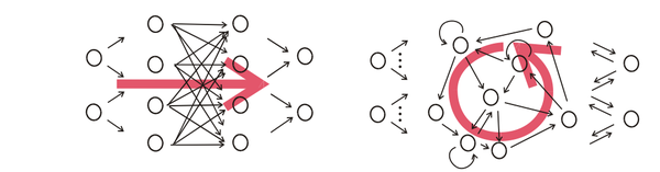图， CNN（左）和 RNN（右）的结构区别， 注意右图中输出和隐变量网络间的双向箭头不一定存在，往往只有隐变量到输出的箭头。

编辑于 2016-11-29

Leon

公众号：智能学之家

一、深度学习：

深度学习是机器学习的一个分支。可以理解为具有多层结构的模型。

二、基本模型：

给大家总结一下深度学习里面的基本模型。我将这些模型大致分为了这几类：多层感知机模型；深度神经网络模型和递归神经网络模型。

2.1 多层感知机模型（也就是你这里说的深度神经网络）：

2.1.1 Stacked Auto-Encoder 堆叠自编码器

堆叠自编码器是一种最基础的深度学习模型，该模型的子网络结构自编码器通过假设输出与输入是相同的来训练调整网络参数，得到每一层中的权重。通过堆叠多层自编码网络可以得到输入信号的几种不同表征（每一层代表一种表征），这些表征就是特征。自动编码器就是一种尽可能复现输入信号的神经网络。为了实现这种复现，自编码器就必须捕捉可以代表输入数据的最重要的因素，就像 PCA 那样，找到可以代表原信息的主要成分。

2.1.1.1 网络结构

堆叠自编码器的网络结构本质上就是一种普通的多层神经网络结构。

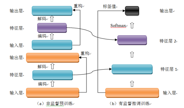
图 1 自编码器网络结构

2.1.1.2 训练过程

堆叠自编码器与普通神经网络不同之处在于其训练过程，该网络结构训练主要分两步：非监督预训练和有监督微调训练。

（1）非监督预训练

自编码器通过自学习得到原始数据的压缩和分布式表征，一般用于高层特征提取与数据非线性降维。结构上类似于一个典型的三层 BP 神经网络，由一个输入层，一个中间隐含层和一个输出层构成。但是，输出层与输入层的神经元个数相等，且训练样本集合的标签值为输入值，即无标签值。输入层到隐含层之间的映射称为编码（Encoder），隐含层到输出层之间的映射称为解码（Decoder）。非监督预训练自编码器的中间层为特征层，在训练好第一层特征层后，第二层和第一层的训练方式相同。我们将第一层输出的特征层当成第二层的输入层，同样最小化重构误差，就会得到第二层的参数，并且得到第二层输入的特征层，也就是原输入信息的第二个表征。以此类推可以训练其他特征层。

（3）有监督微调训练

经过上面的训练方法，可以得到一个多层的堆叠自编码器，每一层都会得到原始输入的不同的表达。到这里，这个堆叠自编码器还不能用来分类数据，因为它还没有学习如何去连结一个输入和一个类。它只是学习获得了一个可以良好代表输入的特征，这个特征可以最大程度上代表原输入信号。那么，为了实现分类，我们就可以在 AutoEncoder 的最顶的编码层添加一个分类器（例如逻辑斯蒂回归、SVM 等），然后通过标准的多层神经网络的监督训练方法（梯度下降法）微调训练。

2.1.1.3 典型改进

（1）Sparse AutoEncoder 稀疏自编码器

在 AutoEncoder 的基础上加上 L1 的稀疏限制（L1 主要是约束每一层中的节点中大部分都要为 0，只有少数不为 0，这就是 Sparse 名字的来源）来减小过拟合的影响，我们就可以得到稀疏自编码器。

（2）Denoising AutoEncoders 降噪自编码器

降噪自动编码器是在自动编码器的基础上，训练数据加入噪声，所以自动编码器必须学习去去除这种噪声而获得真正的没有被噪声污染过的输入。因此，这就迫使编码器去学习输入信号的更加鲁棒的表达，这也是它的泛化能力比一般编码器强的原因。

2.1.1.4 模型优缺点

(1) 优点：

（1）、可以利用足够多的无标签数据进行模型预训练；

（2）、具有较强的数据表征能力。

(2) 缺点：

（1）、因为是全连接网络，需要训练的参数较多，容易出现过拟合；深度模型容易出现梯度消散问题。

（2）、要求输入数据具有平移不变性。

2.1.2、Deep belief network 深度信念网络

2006 年，Geoffrey Hinton 提出深度信念网络（DBN）及其高效的学习算法，即 Pre-training+Fine tuning，并发表于《Science》上，成为其后深度学习算法的主要框架。DBN 是一种生成模型，通过训练其神经元间的权重，我们可以让整个神经网络按照最大概率来生成训练数据。所以，我们不仅可以使用 DBN 识别特征、分类数据，还可以用它来生成数据。

2.1.2.1 网络结构

深度信念网络（DBN）由若干层受限玻尔兹曼机（RBM）堆叠而成，上一层 RBM 的隐层作为下一层 RBM 的可见层。下面先介绍 RBM，再介绍 DBN。

（1） RBM

图 2 RBM 网络结构

一个普通的 RBM 网络结构如上图所示，是一个双层模型，由 m 个可见层单元及 n 个隐层单元组成，其中，层内神经元无连接，层间神经元全连接，也就是说：在给定可见层状态时，隐层的激活状态条件独立，反之，当给定隐层状态时，可见层的激活状态条件独立。这保证了层内神经元之间的条件独立性，降低概率分布计算及训练的复杂度。RBM 可以被视为一个无向图模型，可见层神经元与隐层神经元之间的连接权重是双向的，即可见层到隐层的连接权重为 W，则隐层到可见层的连接权重为 W’。除以上提及的参数外，RBM 的参数还包括可见层偏置 b 及隐层偏置 c。

RBM 可见层和隐层单元所定义的分布可根据实际需要更换，包括：Binary 单元、Gaussian 单元、Rectified Linear 单元等，这些不同单元的主要区别在于其激活函数不同。

（2） DBN

图 3 DBN 模型结构

DBN 模型由若干层 RBM 堆叠而成，如果在训练集中有标签数据，那么最后一层 RBM 的可见层中既包含前一层 RBM 的隐层单元，也包含标签层单元。假设顶层 RBM 的可见层有 500 个神经元，训练数据的分类一共分成了 10 类，那么顶层 RBM 的可见层有 510 个显性神经元，对每一训练数据，相应的标签神经元被打开设为 1，而其他的则被关闭设为 0。

2.1.2.2 训练过程

DBN 的训练包括 Pre-training 和 Fine tuning 两步，其中 Pre-training 过程相当于逐层训练每一个 RBM，经过 Pre-training 的 DBN 已经可用于模拟训练数据，而为了进一步提高网络的判别性能， Fine tuning 过程利用标签数据通过 BP 算法对网络参数进行微调。

（1） Pre-training

如前面所说，DBN 的 Pre-training 过程相当于逐层训练每一个 RBM，因此进行 Pre-training 时直接使用 RBM 的训练算法。

（2） Fine tuning

建立一个与 DBN 相同层数的神经网络，将 Pre-training 过程获得的网络参数赋给此神经网络，作为其参数的初始值，然后在最后一层后添加标签层，结合训练数据标签，利用 BP 算法微调整个网络参数，完成 Fine tuning 过程。

2.1.2.3 改进模型

DBN 的变体比较多，它的改进主要集中于其组成 “零件” RBM 的改进，下面列举两种主要的变体。（这边的改进模型暂时没有深入研究，所以大概参考网上的内容）

（1） 卷积 DBN（CDBN）

DBN 并没有考虑到图像的二维结构信息，因为输入是简单的将一个图像矩阵转换为一维向量。而 CDBN 利用邻域像素的空域关系，通过一个称为卷积 RBM（CRBM）的模型达到生成模型的变换不变性，而且可以容易得变换到高维图像。

（2） 条件 RBM（Conditional RBM）

DBN 并没有明确地处理对观察变量的时间联系的学习上，Conditional RBM 通过考虑前一时刻的可见层单元变量作为附加的条件输入，以模拟序列数据，这种变体在语音信号处理领域应用较多。

2.1.2.4 典型优缺点

对 DBN 优缺点的总结主要集中在生成模型与判别模型的优缺点总结上。

(1) 优点：

（1）、生成模型学习联合概率密度分布，所以就可以从统计的角度表示数据的分布情况，能够反映同类数据本身的相似度；

（2）、生成模型可以还原出条件概率分布，此时相当于判别模型，而判别模型无法得到联合分布，所以不能当成生成模型使用。

(2) 缺点：

（1）、 生成模型不关心不同类别之间的最优分类面到底在哪儿，所以用于分类问题时，分类精度可能没有判别模型高；

（2）、由于生成模型学习的是数据的联合分布，因此在某种程度上学习问题的复杂性更高。

（3）、要求输入数据具有平移不变性。

2.2、Convolution Neural Networks 卷积神经网络

卷积神经网络是人工神经网络的一种，已成为当前语音分析和图像识别领域的研究热点。它的权值共享网络结构使之更类似于生物神经网络，降低了网络模型的复杂度，减少了权值的数量。该优点在网络的输入是多维图像时表现的更为明显，使图像可以直接作为网络的输入，避免了传统识别算法中复杂的特征提取和数据重建过程。卷积网络是为识别二维形状而特殊设计的一个多层感知器，这种网络结构对平移、比例缩放、倾斜或者共他形式的变形具有高度不变性。

2.2.1 网络结构

卷积神经网络是一个多层的神经网络，其基本运算单元包括：卷积运算、池化运算、全连接运算和识别运算。

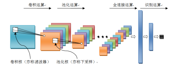
图 4 卷积神经网络结构

l 卷积运算：前一层的特征图与一个可学习的卷积核进行卷积运算，卷积的结果经过激活函数后的输出形成这一层的神经元，从而构成该层特征图，也称特征提取层，每个神经元的输入与前一层的局部感受野相连接，并提取该局部的特征，一旦该局部特征被提取，它与其它特征之间的位置关系就被确定。

l 池化运算：它把输入信号分割成不重叠的区域，对于每个区域通过池化（下采样）运算来降低网络的空间分辨率，比如最大值池化是选择区域内的最大值，均值池化是计算区域内的平均值。通过该运算来消除信号的偏移和扭曲。

l 全连接运算：输入信号经过多次卷积核池化运算后，输出为多组信号，经过全连接运算，将多组信号依次组合为一组信号。

l 识别运算：上述运算过程为特征学习运算，需在上述运算基础上根据业务需求（分类或回归问题）增加一层网络用于分类或回归计算。

2.2.2 训练过程

卷积网络在本质上是一种输入到输出的映射，它能够学习大量的输入与输出之间的映射关系，而不需要任何输入和输出之间的精确的数学表达式，只要用已知的模式对卷积网络加以训练，网络就具有输入输出对之间的映射能力。卷积网络执行的是有监督训练，所以其样本集是由形如：（输入信号，标签值）的向量对构成的。

2.2.3 典型改进

卷积神经网络因为其在各个领域中取得了好的效果，是近几年来研究和应用最为广泛的深度神经网络。比较有名的卷积神经网络模型主要包括 1986 年 Lenet，2012 年的 Alexnet，2014 年的 GoogleNet，2014 年的 VGG，2015 年的 Deep Residual Learning。这些卷积神经网络的改进版本或者模型的深度，或者模型的组织结构有一定的差异，但是组成模型的机构构建是相同的，基本都包含了卷积运算、池化运算、全连接运算和识别运算。

2.2.4 模型优缺点

(1) 优点：

（1）、权重共享策略减少了需要训练的参数，相同的权重可以让滤波器不受信号位置的影响来检测信号的特性，使得训练出来的模型的泛化能力更强；

（2）、池化运算可以降低网络的空间分辨率，从而消除信号的微小偏移和扭曲，从而对输入数据的平移不变性要求不高。

(2) 缺点：

（1）、深度模型容易出现梯度消散问题。

2.3、Recurrent neural network 递归神经网络

在深度学习领域，传统的多层感知机为基础的上述各网络结构具有出色的表现，取得了许多成功，它曾在许多不同的任务上 —— 包括手写数字识别和目标分类上创造了记录。但是，他们也存在一定的问题，上述模型都无法分析输入信息之间的整体逻辑序列。这些信息序列富含有大量的内容，信息彼此间有着复杂的时间关联性，并且信息长度各种各样。这是以上模型所无法解决的，递归神经网络正是为了解决这种序列问题应运而生，其关键之处在于当前网络的隐藏状态会保留先前的输入信息，用来作当前网络的输出。

许多任务需要处理序列数据，比如 Image captioning, speech synthesis, and music generation 均需要模型生成序列数据，其他领域比如 time series prediction, video analysis, and musical information retrieval 等要求模型的输入为序列数据，其他任务比如机器翻译，人机对话，controlling a robot 的模型要求输入输出均为序列数据。

2.3.1 网络结构

图 4.1 左侧是递归神经网络的原始结构，如果先抛弃中间那个令人生畏的闭环，那其实就是简单 “输入层 => 隐藏层 => 输出层” 的三层结构，但是图中多了一个非常陌生的闭环，也就是说输入到隐藏层之后，隐藏层还会输入给自己，使得该网络可以拥有记忆能力。我们说递归神经网络拥有记忆能力，而这种能力就是通过 W 将以往的输入状态进行总结，而作为下次输入的辅助。可以这样理解隐藏状态：

h=f (现有的输入 + 过去记忆总结)

图 5 递归神经网络结构图

2.3.2 训练过程

递归神经网络中由于输入时叠加了之前的信号，所以反向传导时不同于传统的神经网络，因为对于时刻 t 的输入层，其残差不仅来自于输出，还来自于之后的隐层。通过反向传递算法，利用输出层的误差，求解各个权重的梯度，然后利用梯度下降法更新各个权重。

2.3.3 典型改进

递归神经网络模型可以用来处理序列数据，递归神经网络包含了大量参数，且难于训练（时间维度的梯度消散或梯度爆炸），所以出现一系列对 RNN 优化，比如网络结构、求解算法与并行化。今年来 bidirectional RNN （BRNN）与 LSTM 在 image captioning, language translation, and handwriting recognition 这几个方向上有了突破性进展 。

2.3.4 模型优缺点

(1) 优点：

（1）、模型是时间维度上的深度模型，可以对序列内容建模；

(2) 缺点：

（1）、需要训练的参数较多，容易出现梯度消散或梯度爆炸问题；

（2）、不具有特征学习能力。

编辑于 2017-04-13

张蕊

UCLA 想辍学

CNN 专门解决图像问题的，可用把它看作特征提取层，放在输入层上，最后用 MLP 做分类。

RNN 专门解决时间序列问题的，用来提取时间序列信息，放在特征提取层（如 CNN）之后。

DNN 说白了就是 多层网络，只是用了很多技巧，让它能够 deep 。

工具及教程：
http://tensorlayer.readthedocs.io

https://www.tensorflow.org/versions/r0.9/tutorials/index.html

不用谢

编辑于 2016-08-23

魏秀参

1

南京大学 计算机科学与技术博士在读

蟹妖，可参阅我关于深度学习入门的回答。
深度学习入门必看的书和论文？有哪些必备的技能需学习？ - 魏秀参的回答

编辑于 2015-08-20

知乎用户

在序列信号的应用上，CNN 是只响应预先设定的信号长度（输入向量的长度），RNN 的响应长度是学习出来的。

CNN 对特征的响应是线性的，RNN 在这个递进方向上是非线性响应的。这也带来了很大的差别。

编辑于 2016-08-08

知乎用户

我个人的看法是，DNN 是深度学习思想的一个统称，狭义上它是一种逐层贪婪无监督的学习方法，注意它只是一种思想，需要依赖具体的模型去实现，即深度学习 = 逐层贪婪无监督方法 + 特定深度学习模型。而具体的深度学习模型有 CNN、RNN、SDA、RBM、RBM 等。逐层贪婪无监督的深度学习思想是 2006 年提出来的，能有效解决深层网络结构训练的梯度弥散等问题。而 CNN 等网络模型其实很早就提出来了，之前用 BP 之类的老方法效果一直不太好，等到深度学习思想提出来后，这些老模型就都焕发了新生，带来了今天深度学习的火热。回归到问题上来，就是 CNN、RNN、DNN 不是一个层次上的东西，分别是具体的模型和通用的思想。这是我的个人理解，还在学习中，如有错误欢迎指出。

编辑于 2016-02-13

知乎用户

DNN 以神经网络为载体，重在深度，可以说是一个统称。
RNN，回归型网络，用于序列数据，并且有了一定的记忆效应，辅之以 lstm。
CNN 应该侧重空间映射，图像数据尤为贴合此场景。

发布于 2015-08-31

知乎用户

中文不好解释，用英文试试，不当之处请谅解。

Artificial neural networks use networks of activation units (hidden units) to map inputs to outputs. The concept of deep learning applied to this model allows the model to have multiple layers of hidden units where we feed output from the previous layers. However, dense connections between the layers is not efficient, so people developed models that perform better for specific tasks.

The whole "convolution" in convolutional neural networks is essentially based on the fact that we''re lazy and want to exploit spatial relationships in images. This is a huge deal because we can then group small patches of pixels and effectively "downsample" the image while training multiple instances of small detectors with those patches. Then a CNN just moves those filters around the entire image in a convolution. The outputs are then collected in a pooling layer. The pooling layer is again a down-sampling of the previous feature map. If we have activity on an output for filter a, we don''t necessarily care if the activity is for (x, y) or (x+1, y), (x, y+1) or (x+1, y+1), so long as we have activity. So we often just take the highest value of activity on a small grid in the feature map called max pooling.

If you think about it from an abstract perspective, the convolution part of a CNN is effectively doing a reasonable way of dimensionality reduction. After a while you can flatten the image and process it through layers in a dense network. Remember to use dropout layers! (because our guys wrote that paper :P)

I won''t talk about RNN for now because I don''t have enough experience working with them and according to my colleague nobody really knows what''s going on inside an LSTM...but they''re insanely popular for data with time dependencies.

Let''s talk RNN. Recurrent networks are basically neural networks that evolve through time. Rather than exploiting spatial locality, they exploit sequential, or temporal locality. Each iteration in an RNN takes an input and it''s previous hidden state, and produces some new hidden state. The weights are shared in each level, but we can unroll an RNN through time and get your everyday neural net. Theoretically RNN has the capacity to store information from as long ago as possible, but historically people always had problems with the gradients vanishing as we go back further in time, meaning that the model can''t be differentiated numerically and thus cannot be trained with backprop. This was later solved in the proposal of the LSTM architecture and subsequent work, and now we train RNNs with BPTT (backpropagation through time). Here''s a link that explains LSTMs really well: http://colah.github.io/posts/2015-08-Understanding-LSTMs/

Since then RNN has been applied in many areas of AI, and many are now designing RNN with the ability to extract specific information (read: features) from its training examples with attention-based models.

编辑于 2016-02-15

张戎

数学 话题的优秀回答者

之前写过一篇关于 RNN 的文章：循环神经网络－Recurrent Neural Networks

循环神经网络（Recurrent Neural Networks）是目前非常流行的神经网络模型，在自然语言处理的很多任务中已经展示出卓越的效果。但是在介绍 RNN 的诸多文章中，通常都是介绍 RNN 的使用方法和实战效果，很少有文章会介绍关于该神经网络的训练过程。

循环神经网络是一个在时间上传递的神经网络，网络的深度就是时间的长度。该神经网络是专门用来处理时间序列问题的，能够提取时间序列的信息。如果是前向神经网络，每一层的神经元信号只能够向下一层传播，样本的处理在时刻上是独立的。对于循环神经网络而言，神经元在这个时刻的输出可以直接影响下一个时间点的输入，因此该神经网络能够处理时间序列方面的问题。

本文将会从数学的角度展开关于循环神经网络的使用方法和训练过程，在本文中，会假定读者已经掌握数学分析中的导数，偏导数，链式法则，梯度下降法等基础内容。本文将会使用传统的后向传播算法（Back Propagation）来训练 RNN 模型。

发布于 2016-11-19

知乎用户

CNN 就是全连接权值太多，取的一个折衷策略，只取部分连接边扫描一遍整个输入，最后再汇总（求 max 等等操作）。
RNN 就是在隐层加入了自连边和互连边（即隐层可以相互连接），可以按时序展开为一系列 FNN。常见训练算法为 bptt 和 lstm。
DNN 个人理解就是隐层有很多层，bp 反传时可能梯度会锐减或剧增，导致误差传不回来，可以通过重新设计网络结构（类似 lstm）的办法来解决。

发布于 2015-08-18

知乎用户

想学专业知识就要少上知户 多看书

Stanford University CS231n: Convolutional Neural Networks for Visual Recognition

编辑于 2016-02-15

Gundam

The truth is what it is, not what u c 09

DNN 区别于浅层神经网络，是所有深度学习中的网络模型统称，包括 CNN、RNN 等，以后还会有新的网络模型提出。题主说的 CNN 应该是三大特点：local receptive fields、shared weights 和 pooling。他们的用途都是拿数据来训练学习特征（太笼统了，嘿嘿），省去手工提取特征的过程，类似是一个通用的学习框架。

@helloworld00

回答中提到的课程不错，针对卷积神经网络和视觉识别的，题主可以深入学习一下。UFLDL 也很适合初学者。另外如果真想研究深度学习，还是要看论文的 -->Reading List « Deep Learning

关于神经网络 参数计算--直接解析CKPT文件读取和神经网络checkpoint的介绍现已完结，谢谢您的耐心阅读，如果想了解更多关于01.神经网络和深度学习 W3.浅层神经网络（作业：带一个隐藏层的神经网络）、01.神经网络和深度学习 W4.深层神经网络（作业：建立你的深度神经网络+图片猫预测）、bp神经网络参数怎么设置,bp神经网络参数设置、CNN (卷积神经网络)、RNN (循环神经网络)、DNN (深度神经网络) 的内部网络结构有什么区别？的相关知识，请在本站寻找。