对于在matplotlib中使用图,轴或图形绘制图之间有什么区别?感兴趣的读者,本文将提供您所需要的所有信息,我们将详细讲解matplotlib双轴图怎么画图标,并且为您提供关于matplotlib中
对于在matplotlib中使用图,轴或图形绘制图之间有什么区别?感兴趣的读者,本文将提供您所需要的所有信息,我们将详细讲解matplotlib双轴图怎么画图标,并且为您提供关于matplotlib中具有标题,轴标签的确切图形大小、matplotlib中的plt.draw和fig.canvas.draw有什么区别?、matplotlib各图形绘制、python – 在matplotlib中绘制一条关联多个子图之间区域的线的宝贵知识。
本文目录一览:- 在matplotlib中使用图,轴或图形绘制图之间有什么区别?(matplotlib双轴图怎么画图标)
- matplotlib中具有标题,轴标签的确切图形大小
- matplotlib中的plt.draw和fig.canvas.draw有什么区别?
- matplotlib各图形绘制
- python – 在matplotlib中绘制一条关联多个子图之间区域的线
")
在matplotlib中使用图,轴或图形绘制图之间有什么区别?(matplotlib双轴图怎么画图标)
当我在matplotlib,tbh中绘制图时,我有点困惑后端的处理方式,我不清楚图,轴和图形的层次结构。我阅读了文档,它很有帮助,但我仍然感到困惑…
以下代码以三种不同的方式绘制相同的图:
#creating the arrays for testingx = np.arange(1, 100)y = np.sqrt(x)#1st wayplt.plot(x, y)#2nd wayax = plt.subplot()ax.plot(x, y)#3rd wayfigure = plt.figure()new_plot = figure.add_subplot(111)new_plot.plot(x, y)现在我的问题是-
这三种方法有什么区别?我的意思是,当调用这三种方法中的任何一种时,幕后情况是什么?
什么时候应该使用哪种方法,在这些方法上使用利弊是什么?
答案1
小编典典方法1
plt.plot(x, y)这样一来,您只能绘制一个具有(x,y)坐标的图形。如果您只想获取一张图形,则可以使用这种方式。
方法二
ax = plt.subplot()ax.plot(x, y)这使您可以在同一窗口中绘制一个或多个图形。在编写时,您将仅绘制一个图形,但是可以进行如下操作:
fig1, ((ax1, ax2), (ax3, ax4)) = plt.subplots(2, 2)您将绘制4个图形,每个图形分别命名为ax1,ax2,ax3和ax4,但在同一窗口上。在我的示例中,此窗口将分为四个部分。
方法3
fig = plt.figure()new_plot = fig.add_subplot(111)new_plot.plot(x, y)我没有使用它,但是可以找到文档。
例:
import numpy as npimport matplotlib.pyplot as plt# Method 1 #x = np.random.rand(10)y = np.random.rand(10)figure1 = plt.plot(x,y)# Method 2 #x1 = np.random.rand(10)x2 = np.random.rand(10)x3 = np.random.rand(10)x4 = np.random.rand(10)y1 = np.random.rand(10)y2 = np.random.rand(10)y3 = np.random.rand(10)y4 = np.random.rand(10)figure2, ((ax1, ax2), (ax3, ax4)) = plt.subplots(2, 2)ax1.plot(x1,y1)ax2.plot(x2,y2)ax3.plot(x3,y3)ax4.plot(x4,y4)plt.show()
matplotlib中具有标题,轴标签的确切图形大小
之前也曾提出过类似的问题,但是我所有的搜索结果都无法解决我的问题。采取以下示例代码:
from matplotlib.pyplot import *fig = figure(1, figsize=(3.25, 3))plot([0,1,5,2,9])title(''title'')xlabel(''xAxis'')ylabel(''yAxis'')fig.savefig(''test.png'',dpi=600)结果数字为2040x1890像素或3.4“
x3.15”,并且x标签被切除。在图像编辑器中查看PNG文件,似乎轴和刻度标签符合所需的大小。我试图从输出大小和请求的大小中获取差异,并将其反馈给(3.25-(3.4-3.25)=
3.10,但是matplotlib似乎添加了一个任意缓冲区,但仍然没有达到所需的大小。如何使整体数字成为所需大小?
答案1
小编典典与David Robinson的评论一致,尽管xlabel确实显示了截断(在python 2.6 64位中的mpl
1.1.0,win7),但通过photoshop测量,此处生成的数字是3.25 x 3英寸(按Photoshop测量)
解决此问题的一种方法是使用以下方法手动调整边距subplot_adjust:
from matplotlib.pyplot import *fig = figure(1, figsize=(3.25, 3))plot([0, 1, 5, 2, 9])title(''title'')xlabel(''xAxis'')ylabel(''yAxis'')subplots_adjust(bottom=0.14) # <--fig.savefig(''test.png'', dpi=600)这些边距的默认值在matploblibrc文件中设置,您可以在那里永久修改它。在我的情况下,下边距的默认值为0.10。
如果您的图形尺寸错误或正确(如我的情况),则可以使用subplot_adjust为标签提供足够的空间。然后,如果需要,您可以计算校正量,以获取所需的实际图片或图形尺寸。
保存的图形的最终视图取决于该图形的大小。如果您show()将图形保存在matplotlib视图框架中,则会在图像中截取标签。但是,如果您手动增加图像的尺寸,则会看到标签出现,如果您保存它,标签也将出现在保存的图像中。可以说是所见即所得。您的图形尺寸很小,这会使您的标签被剪掉。因此,另一种方法是使用较低的dpi制作更大的数字,以保持整体尺寸。这也适用:
from matplotlib.pyplot import *fig = figure(1, figsize=(6.5, 6)) # <---plot([0, 1, 5, 2, 9])title(''title'')xlabel(''xAxis'')ylabel(''yAxis'')fig.savefig(''test.png'', dpi=300) # <---无论如何,我都将其视为matplolib错误,因为您可能希望在绘制和保存后有未切割的图形。

matplotlib中的plt.draw和fig.canvas.draw有什么区别?
如何解决matplotlib中的plt.draw和fig.canvas.draw有什么区别??
我试图在jupyter笔记本中获得动态数字。搜索关于stackexchange和测试的答案后,我发现将plt.draw更改为fig.canvas.draw可以动态绘制图形。使用plt.draw时,整个过程会暂停并在最后显示最终图。为什么使用fig.canvas.draw产生我想要的结果而不是plt.draw?
%matplotlib notebook

import matplotlib.pyplot as plt
import numpy as np
from scipy.stats import norm

n = 5

for n in [1,2,3,4,5]:
    plt.scatter(n,n)
    plt.draw()
    plt.pause(0.5)
%matplotlib notebook

import matplotlib.pyplot as plt
import numpy as np
from scipy.stats import norm

n = 5

fig = plt.figure()
ax = fig.add_subplot(111)

for n in [1,5]:
    ax.scatter(n,n)
    fig.canvas.draw()
    plt.pause(0.5)
解决方法
暂无找到可以解决该程序问题的有效方法,小编努力寻找整理中!
如果你已经找到好的解决方法,欢迎将解决方案带上本链接一起发送给小编。
小编邮箱:dio#foxmail.com (将#修改为@)

matplotlib各图形绘制
2D图形
import numpy as np
import pandas as pd
from pandas import Series,DataFrame
import matplotlib.pyplot as plt
散点图
【散点图需要两个参数x,y,但此时x不是表示x轴的刻度,而是每个点的横坐标!】
scatter()
通过散点图 可以研究 两个特征之间的关系
x = np.random.normal(loc=0,scale=5,size=1000)
y = np.random.normal(loc=0,scale=5,size=1000)
# plt.plot()  # plot绘制的是折线图
plt.scatter(x,y)  #  plt.scatter()绘制的是散点图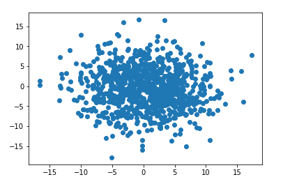
plt.scatter(x,y,s=80,c=''red'') # s size指的是散点的大小 c color指的是散点的颜色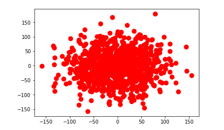
size = np.random.randint(0,100,1000)
color = np.random.random(size=(1000,3))
# 给这1000个点 随机产生 不同的 大小和颜色
plt.scatter(x,y,s=size,c=color,alpha=0.6,marker=''*'')
plt.axis(''off'')
饼图
【饼图也只有一个参数x!】
pie() 饼图适合展示各部分占总体的比例,条形图适合比较各部分的大小
普通各部分占满饼图
data = np.array([30,50,24,80])  # 如果各个值 加起来 比1大 就会计算各个部分的百分比
plt.pie(data)
plt.axis(''equal'')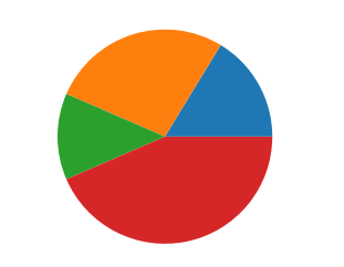
普通未占满饼图
data = np.array([0.2,0.4,0.2,0.1])  # 如果比1 小 直接把各个部分的值 作为 百分比
plt.pie(data)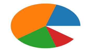
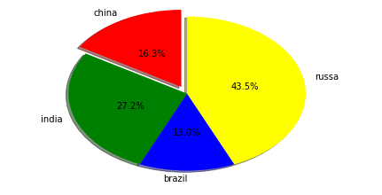
饼图阴影、分裂等属性设置
- labels参数设置每一块的标签;
- labeldistance参数设置标签距离圆心的距离(比例值,只能设置一个浮点小数)
- autopct参数设置比例值的显示格式(%.nf%%);
- pctdistance参数设置比例值文字距离圆心的距离
- explode参数设置每一块顶点距圆形的长度(比例值,列表);
- colors参数设置每一块的颜色(列表);
- shadow参数为布尔值,设置是否绘制阴影
- startangle参数设置饼图起始角度
data = np.array([30,50,24,80])
_ = plt.pie(data
            ,labels=[''china'',''india'',''brazil'',''russa'']  # 各个部分的名字(标签)
            ,labeldistance=1.1  # 标签到中心点的距离
            ,autopct=''%.1f%%''  # 控制比例的值的显示
            ,pctdistance=0.5  # 控制百分比的值的显示位置
            ,explode=[0.1,0,0,0]  # 每一份扇形 到中心点的距离
            ,colors = [''red'',''green'',''blue'',''yellow'']
            ,shadow=True
            ,startangle=90  # 绘制图形时候 开始的角度
           )
直方图
【直方图的参数只有一个x!!!不像条形图需要传入x,y】
hist()的参数
- bins
- 可以是一个bin数量的整数值,也可以是表示bin的一个序列。默认值为10
- density (normed)
- 如果值为True,直方图的值将进行归一化处理,形成概率密度,默认值为False
- color
- 指定直方图颜色。可以是单一色值或颜色序列。如果指定了多个数据集合,颜色序列将会设置为相同的顺序。如果未指定,将会使用一个默认的线条颜色
- orientation
- 通过设置orientation为horizontal创建水平直方图。默认值为vertical
data = np.random.randint(0,100,size=100)
df = DataFrame(data)
df.plot(kind=''hist'')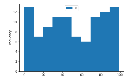
# bins指的是要把整个范围 分成多少份 默认值是10
# density把值从频率变成概率
# orientation用来控制条形图的方向 horizontal表示水平
plt.hist(data,bins=5,density=True,color=''r'',orientation=''horizontal'')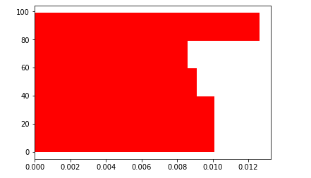
条形图
【条形图有两个参数x,y】
- width 水平方向的长度
- height 竖直方向的长度
bar()、barh()
data = np.array([1,4,7,2,8,5])
index = [1,2,3,4,5,6]
# x是索引, height是高度(值)
plt.bar(x=index,height=data,width=0.5)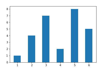
# y是各个样本的索引
# 各个样本的值的大小 用width来体现
plt.barh(y=index,height=0.5,width=data)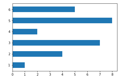
data = np.array([1,2,3,4,5,6])
index = [1,2,3,4,5,6]
plt.bar(x=index,height=data,width=0.5)
plt.axes(polar=True)
data = np.array([1,2,3,4,5,6])
index = [1,2,3,4,5,7]
plt.bar(x=index,height=data,width=0.5)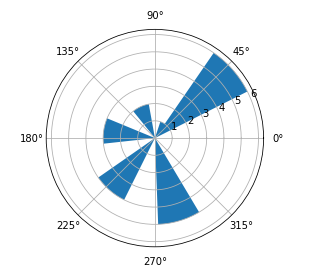
index = np.arange(0,2*np.pi,np.pi/4)
data = [1,2,3,4,5,6,7,8]
plt.axes(polar=True)
plt.bar(x=index,height=data,width=0.5)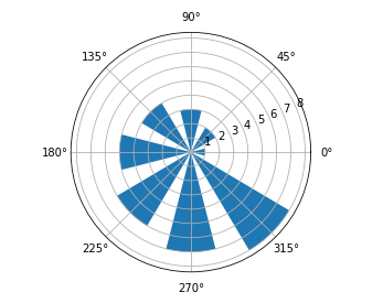
图形内的文字、注释、箭头
控制文字属性的方法:
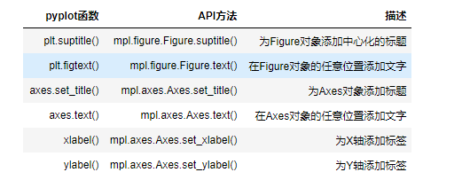
所有的方法会返回一个matplotlib.text.Text对象
图形内的文字
text()
# 以下所有这些 都是文字对象 都可以设置 color rotation fontsize fontproperties ...
axes = plt.subplot()
plt.title(''title'')  # 画布标题 实际上 内部调用的 就是axes坐标系的标题
# plt.suptitle(''suptitle'',color=''r'',rotation=90,fontsize=10)
plt.figtext(0.2,0.8,''fig_text'')  # 画布内的文本 x和y参数用来指定位置(0-1之间 不过也可以超出这个范围) s就是文字的内容
axes.set_title(''axes_title'')
axes.text(0.5,0.5,''axes_text'')  # x, y, s
axes.text(0.8,0.2,''axes_text'')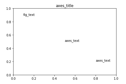
注释
annotate()
- xy参数设置箭头指示的位置
- xytext参数设置注释文字的位置
- arrowprops参数以字典的形式设置箭头的样式
- width参数设置箭头长方形部分的宽度
- headlength参数设置箭头尖端的长度,
- headwidth参数设置箭头尖端底部的宽度
- shrink参数设置箭头顶点、尾部与指示点、注释文字的距离(比例值),可以理解为控制箭头的长度
data = np.random.randint(0,10,size=10)
index = np.arange(0,10,1)
data
index
plt.plot(index,data)
# s 注释的内容
# xy 注释的位置 以列表或者元组的形式 设置x和y的座标(注意 不是0-1的那种值)
# plt.annotate(''hehe'',[5,2])
# 如果想添加 箭头 可以用 arrowprops来设置箭头的样式
# plt.annotate(s=''hehe'',xy=[5,2],xytext=[0,8],arrowprops={''width'':2}) # xytext用来设置文本的位置 xy是箭头指向的位置
# plt.annotate(s=''hehe'',xy=[5,2],xytext=[0,8],arrowprops={''width'':2},color=''r'',rotation=90) # annotation注释 也是文本对象 也可以设置文本属性
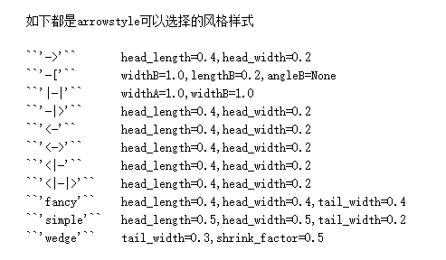
plt.annotate(s=''hehe'',xy=[5,2],xytext=[0,8],arrowprops={''width'':20,''headlength'':25,''headwidth'':25}) # 设置箭头的样式 箭头身体的宽度width 箭头头部的宽度headwidth 长度headlength
plt.plot(index,data)
plt.annotate(s=''hehe'',xy=[5,2],xytext=[0,8],arrowprops={''arrowstyle'':''fancy''})
3D图
曲面图
导包
- from mpl_toolkits.mplot3d.axes3d import Axes3D
使用mershgrid函数切割x,y轴
- X,Y = np.meshgrid(x, y)
创建3d坐标系
- axes = plt.subplot(projection=''3d'')
绘制3d图形
- p = axes.plot_surface(X,Y,Z,color=''red'',cmap=''summer'') # 返回图形对象
添加colorbar
- plt.colorbar(p,shrink=0.5) # 传入图形对象
from mpl_toolkits.mplot3d.axes3d import Axes3D
axes = plt.subplot(projection=''3d'')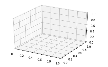
# 取遍 x y 平面上的整数点
x = np.linspace(0,5,6)  # 取遍了x轴线上的整数点
x
y = np.linspace(0,5,6)
y
X,Y = np.meshgrid(x,y)def fn(x,y):
return np.sin(y)-np.cos(x)
Z = fn(X,Y)
x = np.linspace(-6,6,100)
y = np.linspace(-6,6,100)
X,Y = np.meshgrid(x,y)
# plot_surface绘制平面
plt.figure(figsize=(12,8))
axes = plt.subplot(projection=''3d'')
# axes.plot_surface(X, Y, Z,color=''red'')
p = axes.plot_surface(X, Y, Z,cmap=''rainbow'')
plt.colorbar(p,shrink=0.5)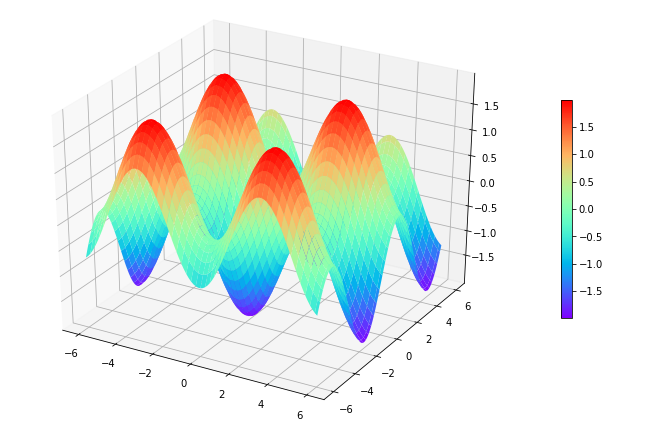
玫瑰图/极坐标条形图
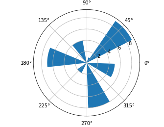
创建极坐标,设置polar属性
plt.axes(polar = True)
绘制极坐标条形图
index = np.arange(0,2*np.pi,2*np.pi/8)
plt.bar(x=index ,height = [1,2,3,4,5,6,7,8] ,width = 2*np.pi/8)

python – 在matplotlib中绘制一条关联多个子图之间区域的线
我是一名地质学家,有一堆不同深度的钻孔.
我粗略地设定了子图的数量,宽度和高度,以根据钻孔的数量和这些钻孔中的样本数量而变化.
在每个钻孔中都有一个我想要突出显示的区域,我用axhspan完成了这个区域.
我想做的是在钻孔(子图)之间进行关联,绘制一条连接所有钻孔区域顶部和底部的线.
我尝试过使用注释但没有取得很大进展.
我不确定如何处理这个问题,并且不胜感激.
这是一些示例代码,以及它可能产生的图片
import numpy as np
import matplotlib.pyplot as plt
from random import randint

fig = plt.figure()

Wells=np.arange(0,10,1) #number of wells to plot

for i in Wells:
    samp=randint(50,100) #number of samples in well

    dist=0.02     #space between plots
    left=0.05     #left border
    right=0.05    #right border
    base=0.05     #bottom border
    width=((1.0-(left+right))/len(Wells))     #width of subplot
    height=(1.0-base)/(100.0/samp)            #height of subplot

    #create subplots
    ax = fig.add_axes([left+(i*width)+dist,1.0-(base+height),width-dist,height])    #left,bottom,width,height of subplot

    #random data
    x=np.random.random_integers(100,size=(samp))
    y=np.arange(0,len(x),1)

    #plot
    ax.plot(x,y,alpha=0.5)

    #zone area of plot
    zone=samp/2.5
    ax.axhspan(15,zone,color='k',alpha=0.2) #axis 'h' horizontal span

    #format
    ax.set_ylim(0,max(y))
    ax.set_xlim(0,max(x))
    ax.tick_params(axis='both',label1On=False,label2On=False)

plt.show()
:
在for循环之前添加:
xys_bot = []
xys_top = []
在for循环结束时:
for i in Wells:
    #
    #...
    #
    xys_bot.append( ((x.max() - x.min())/2.,15) )
    xys_top.append( ((x.max() - x.min())/2.,zone) )
    if i > 0:
        # bottom line
        p = ConnectionPatch(xyA = xys_bot[i-1],xyB = xys_bot[i],coordsA='data',coordsB='data',axesA=fig.axes[i-1],axesB=ax,arrow)
        ax.add_artist(p)
        # top line
        p = ConnectionPatch(xyA = xys_top[i-1],xyB = xys_top[i],arrow)
        ax.add_artist(p)

plt.draw()
plt.show()
今天关于在matplotlib中使用图,轴或图形绘制图之间有什么区别?和matplotlib双轴图怎么画图标的介绍到此结束,谢谢您的阅读,有关matplotlib中具有标题,轴标签的确切图形大小、matplotlib中的plt.draw和fig.canvas.draw有什么区别?、matplotlib各图形绘制、python – 在matplotlib中绘制一条关联多个子图之间区域的线等更多相关知识的信息可以在本站进行查询。
本文标签:


![[转帖]Ubuntu 安装 Wine方法(ubuntu如何安装wine)](https://www.gvkun.com/zb_users/cache/thumbs/4c83df0e2303284d68480d1b1378581d-180-120-1.jpg)