本文将为您提供关于SearchingforMobileNetV3的详细介绍，同时，我们还将为您提供关于2017-ICLR-NeuralArchitectureSearchwithReinforceme

本文将为您提供关于Searching for MobileNetV3的详细介绍，同时，我们还将为您提供关于2017-ICLR-Neural Architecture Search with Reinforcement Learning 论文阅读、Angular module 的 forRoot 和 forChild 方法、ArcGIS for Windows Mobile 3.1发布、Creating a Connection Between Enterprise Search and SAP HANA for ABAP CDS-Based Search Models的实用信息。

本文目录一览：

• Searching for MobileNetV3
• 2017-ICLR-Neural Architecture Search with Reinforcement Learning 论文阅读
• Angular module 的 forRoot 和 forChild 方法
• ArcGIS for Windows Mobile 3.1发布
• Creating a Connection Between Enterprise Search and SAP HANA for ABAP CDS-Based Search Models

Searching for MobileNetV3

2017-ICLR-Neural Architecture Search with Reinforcement Learning 论文阅读

NAS with RL

2017-ICLR-Neural Architecture Search with Reinforcement Learning

Google Brain
Quoc V . Le etc
GitHub： stars
Citation：1499

Abstract

we use a recurrent network to generate the model descriptions of neural networks and train this RNN with reinforcement learning to maximize the expected accuracy of the generated architectures on a validation set.

用RNN生成模型描述（边长的字符串），用RL（强化学习）训练RNN，来最大化模型在验证集上的准确率。

Motivation

Along with this success is a paradigm shift from feature designing to architecture
designing,
深度学习的成功是因为范式的转变：特征设计（SIFT、HOG）到结构设计（AlexNet、VGGNet）。

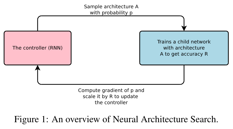
This paper presents Neural Architecture Search, a gradient-based method for finding good architectures (see Figure 1) .

控制器RNN生成很多网络结构（用变长字符串描述），以p的概率采样出结构A，训练网络A，得到准确率R，计算p的梯度，and scale it by R* to update the controller(RNN).

Our work is based on the observation that the structure and connectivity of a neural network can be typically specified by a variable-length string.
观察到网络结构和连接可以可以表示为变长的字符串。

It is therefore possible to use a recurrent network – the controller – to generate such string.
变长字符串可以用RNN（控制器）来生成。

Training the network specified by the string – the “child network” – on the real data will result in an accuracy on a validation set.
训练特定的字符串（子网络），在验证集上，得到验证集准确率。

Using this accuracy as the reward signal, we can compute the policy gradient to update the controller.
使用验证集准确率作为奖励，更新控制器RNN。

As a result, in the next iteration, the controller will give higher probabilities to architectures that receive high accuracies. In other words, the controller will learn to improve its search over time.
在下一个迭代中，控制器RNN生成准确率高的结构的概率会更大。就是说控制器RNN会学会不断改进搜索（生成）策略，以生成更好地结构。

Contribution

将卷积网络结构描述为变长的字符串
使用RNN控制器来生成变长的字符串
使用准确率来更新RNN使得生成的结构（字符串）质量越来越高

Method

3.1 GENERATE MODEL DESCRIPTIONS WITH A CONTROLLER RECURRENT NEURAL NETWORK

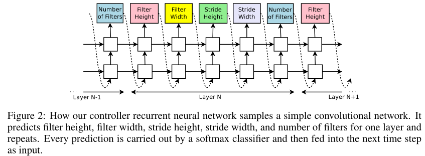
Let’s suppose we would like to predict feedforward neural networks with only convolutional layers, we can use the controller to generate their hyperparameters as a sequence of tokens:
设我们要预测（生成/搜索）的前向网络是卷积网络，我们可以用控制器RNN来生成每一层的超参数（序列）：（卷积核高、宽，stride 高、宽，卷积核数量）五元组

In our experiments, the process of generating an architecture stops if the number of layers exceeds a certain value.
根据经验，层数超过特定值的时候，生成结构的过程将会停止。**层数从少到多？最后都是生成指定层的结构？

This value follows a schedule where we increase it as training progresses.
这个指定值随着训练过程逐渐增加。

Once the controller RNN finishes generating an architecture, a neural network with this architecture is built and trained.
一旦控制器RNN完成一个结构的生成，该结构的网络已经建立并且被训练完毕**。

At convergence, the accuracy of the network on a held-out validation set is recorded.
（子网络训练**）收敛时，记录验证集上的准确率。

The parameters of the controller RNN, θc, are then optimized in order to maximize the expected validation accuracy of the proposed architectures.
根据验证集准确率更新控制器RNN，参数θc。

In the next section, we will describe a policy gradient method which we use to update parameters θc so that the controller RNN generates better architectures over time.
下一部分继续阐述如何根据梯度策略更新控制器RNN的参数θc

3.2 Training with Reinforce

The list of tokens that the controller predicts can be viewed as a list of actions \(a_{1:T}\) to design an architecture for a child network.
控制器RNN生成的代表子网络的序列可以写为\(a_{1:T}\).

At convergence, this child network will achieve an accuracy R on a held-out dataset.
子网络训练到收敛时，会得到在验证集上的准确率R

We can use this accuracy R as the reward signal and use reinforcement learning to train the controller.
我们可以使用R作为训练RNN控制器的奖励

More concretely, to find the optimal architecture, we ask our controller to
maximize its expected reward, represented by \(J(θ_c)\):
具体地，我们让控制器最大化奖励R的期望，期望可以表示为\(J(θ_c)\):
\(J\left(\theta_{c}\right)=E_{P\left(a_{1: T} ; \theta_{c}\right)}[R]\).
⭐️ **如何计算R的期望？\(P\left(a_{1: T} ; \theta_{c}\right)\),是什么？

Since there ward signal R is non-differentiable, we need to use a policy gradient method to iteratively update \(θ_c\).
由于R是不可微的，所以我们使用梯度方法来迭代更新\(θ_c\).
\(\nabla_{\theta_{c}} J\left(\theta_{c}\right)=\sum_{t=1}^{T} E_{P\left(a_{1: T} ; \theta_{c}\right)}\left[\nabla_{\theta_{c}} \log P\left(a_{t} | a_{(t-1): 1} ; \theta_{c}\right) R\right]\).
⭐️ **\(P\left(a_{t} | a_{(t-1): 1} ; \theta_{c}\right)\).是什么？\(\sum_{t=1}^{T}\).又是什么？

An empirical approximation of the above quantity is:
上述等式右边根据经验近似为：
\(\frac{1}{m} \sum_{k=1}^{m} \sum_{t=1}^{T} \nabla_{\theta_{c}} \log P\left(a_{t} | a_{(t-1): 1} ; \theta_{c}\right) R_{k}\).
⭐️ 怎么近似的？

Where m is the number of different architectures that the controller samples in one batch and T is the number of hyperparameters our controller has to predict to design a neural network architecture.
公式中m是不同结构的数量，T是控制结构的序列的长度（超参的数量）

The validation accuracy that the k-th neural network architecture achieves after being trained on a training dataset is \(R_k\).
\(R_k\)是第k个结构的训练精度

The above update is an unbiased estimate for our gradient, but has a very high variance. In order to reduce the variance of this estimate we employ a baseline function:
以上是梯度的无偏估计，但⭐️方差较大？，我们将其剪去baseline
\(\frac{1}{m} \sum_{k=1}^{m} \sum_{t=1}^{T} \nabla_{\theta_{c}} \log P\left(a_{t} | a_{(t-1): 1} ; \theta_{c}\right)\left(R_{k}-b\right)\)

As long as the baseline function b does not depend on the on the current action, then this is still an unbiased gradient estimate.
只要baseline不依赖当前值，就仍然是无偏估计

In this work, our baseline b is an exponential moving average of the previous architecture accuracies.
具体地，baseline的值b为先前结构的指数移动平均值（EMA）

In Neural Architecture Search, each gradient update to the controller parameters \(θ_c\) corresponds to training one child net-work to convergence.
⭐️ 每次训练一个子网络到收敛时才更新控制器RNN的梯度？

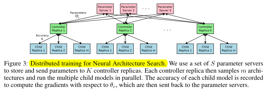
As training a child network can take hours, we use distributed training and asynchronous parameter updates in order to speed up the learning process of the controller (Dean et al., 2012).
训练一个子网络花费几个小时，我们使用分布式训练来加速控制器RNN的学习

We use a parameter-server scheme where we have a parameter server of S shards, that store the shared parameters for K controller replicas.
我们使用parameter-server的策略进行分布式训练....

3.3 Increase Architecture Complexity Skip Connections and Other Layer Types

In Section 3.1, the search space does not have skip connections, or branching layers used in modern architectures such as GoogleNet (Szegedy et al., 2015), and Residual Net (He et al., 2016a).
在3.1节中，搜索空间只有卷积层，没有skip connection(ResNet)，branching layers(GoogLeNet)

In this section we introduce a method that allows our controller to propose skip connections or branching layers, thereby widening the search space.
这一节中，我们允许控制器RNN提出skip connections 和 branch layers，即扩大搜索空间

To enable the controller to predict such connections, we use a set-selection type attention (Neelakan-tan et al., 2015) which was built upon the attention mechanism (Bahdanau et al., 2015; Vinyals et al., 2015).
为了让控制器RNN预测这些新的连接，我们使用了一种​ ⭐️ 注意力机制（集合选择型注意力？）

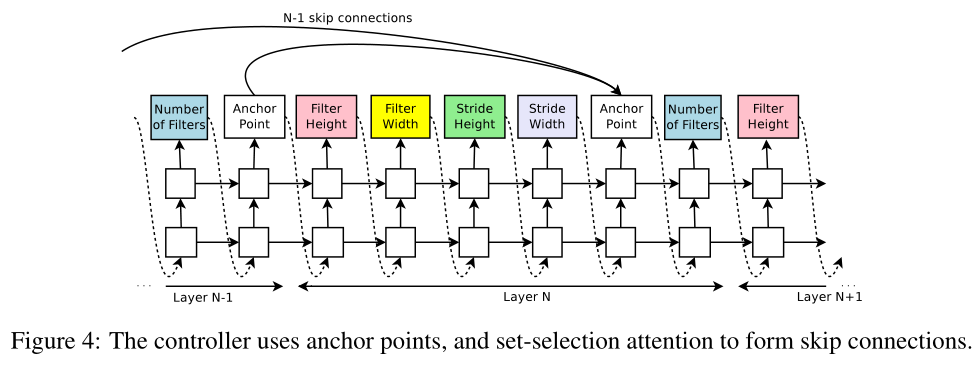
At layer N, we add an anchor point which has N − 1 content-based sigmoids to indicate the previous layers that need to be connected.
在第N层，我们添加N-1个anchor point ⭐️ ，anchor point是基于content 的sigmoids 函数，来指示之前的N-1个层是否需要连接到当前层

Each sigmoid is a function of the current hiddenstate of the controller and the previous hiddenstates of the previous N − 1 anchor points:
每个sigmoid函数是控制器RNN当前隐藏状态 和 之前N-1个anchor points隐藏状态的函数，第 \(i/N\) 层的sigmoid函数可以表示为：
\(\mathrm{P}(\text { Layer } \mathrm{j} \text { is an input to layer } \mathrm{i})=\operatorname{sigmoid}\left(v^{\mathrm{T}} \tanh \left(W_{\text {prev}} * h_{j}+W_{\text {curr}} * h_{i}\right)\right)\)

where \(h_j\) represents the hiddenstate of the controller at anchor point for the j-th layer, where j ranges from 0 to N − 1.
式中 \(h_j\) 表示控制器RNN第 \(j\) 层anchor point的隐藏状态，\(j∈[0, N-1]\)

We then sample from these sigmoids to decide what previous layers to be used as inputs to the current layer.
我们从这些sigmoids中采样，以决定将先前的哪个层作为当前层的输入

The matrices \(W_{prev}\), \(W_{currand}\) ,\(v\) are trainable parameters.

As these connections are also definedby probability distributions, the REINFORCE method still applies without any significant modifications.
在这些连接中，我们一样定义概率分布，强化（学习）的方法依然应用，无需额外修改

Figure 4 shows how the controller uses skip connections to decide what layers it wants as inputs to the current layer.

In our framework, if one layer has many input layers then all input layers are concatenated in the depth dimension.
如果有多个input layer，那么这些input在depth维度上concatenated

Skip connections can cause “compilation failures” where one layer is not compatible with another layer, or one layer may not have any input or output. To circumvent these issues, we employ three simple techniques.
skip connections会导致concatenated失败，比如不同层的output维度不同、一个层没有input或没有output，为了解决这个问题，我们使用了3个技术

First, if a layer is not connected to any input layer then the image is used as the input layer.
一，如果一个层没有input layer，那么把image作为input layer

Second, at the final layer we take all layer outputs that have not been connected and concatenate them before sending this final hidden state to the classifier.
二，在最后一层，我们将之前所有没有output layer的层的outputs concatenate，作为最后一层的输入/ ⭐️ 隐藏状态？

Lastly, if input layers to be concatenated have different sizes, we pad the small layers with zeros so that the concatenated layers have the same sizes.
三，如果需要concatenate的多个input layers的维度不同，用zeros padding小的input使维度统一

Finally, in Section 3.1, we do not predict the learning rate and we also assume that the architectures consist of only convolutional layers, which is also quite restrictive.
在3.1节中，我们不预测learning rate，且假设网络只包含卷积层，限制很严格

It is possible to add the learning rate as one of the predictions.
加上对learning rate的预测

Additionally, it is also possible to predict pooling, local contrast normalization (Jarrett et al., 2009; Krizhevsky et al., 2012), and batchnorm (Ioffe & Szegedy, 2015) in the architectures.
此外，也可以加上对pooling，LCN（局部对比度归一化），bn层的预测

To be able to add more types of layers, we need to add an additional step in the controller RNN to predict the layer type, then other hyperparameters associated with it.
为了增加更多层类型，我们需要在控制器RNN增加额外的步骤，以及额外的超参数（来表示新的层）

Experiments

We apply our method to an image classification task with CIFAR-10

On CIFAR-10, our goal is to find a good convolutional architecture

. On each dataset, we have a separate held-out validation dataset to compute the reward signal.

The reported performance on the test set is computed only once for the network that achieves the best result on the held-out validation dataset.

Search space: Our search space consists of convolutional architectures, with rectified linear units(ReLU) as non-linearities (Nair & Hinton, 2010), batch normalization (Ioffe & Szegedy, 2015) and skip connections between layers (Section 3.3).
搜索空间：卷积结构，包含ReLU、BN、skip connections

For every convolutional layer, the controller RNN has to select a filter height in [1, 3, 5, 7], a filter width in [1, 3, 5, 7], and a number of filters in [24, 36, 48, 64]. For strides, we perform two sets of experiments, one where we fix the strides to be 1, and one where we allow the controller to predict the strides in [1, 2, 3].
具体的搜索空间：filter height[1 3 5 7], weight[1 3 5 7], num[24 36 48 67]，stride[1] or [1 2 3]

Training details: The controller RNN is a two-layer LSTM with 35 hidden units on each layer. It is trained with the ADAM optimizer (Kingma & Ba, 2015) with a learning rate of 0.0006. The weights of the controller are initialized uniformly between -0.08 and 0.08.

trained on 800 GPUs concurrently at any time.
同时在800块GPU上训练

Once the controller RNN samples an architecture, a child model is constructed and trained for 50 epochs.

The reward used for updating the controller is the maximum validation accuracy of the last 5 epochs cubed.
过去5个epochs的最高测试集精度作为更新控制器RNN的奖励

The validation set has 5,000 examples randomly sampled from the training set, the remaining 45,000 examples are used for training.
从5w个训练集样本中抽5000个作为验证集，剩下45000个作为训练集

We use the Momentum Optimizer with a learning rate of 0.1, weight decay of 1e-4, momentum of 0.9 and used Nesterov Momentum
定义Optimizer，weight decay，momentum

During the training of the controller, we use a schedule of increasing number of layers in the child networks as training progresses.
随着训练过程进行，逐渐增加网络层数

On CIFAR-10, we ask the controller to increase the depth by 2 for the child models every 1,600 samples, starting at 6 layers.
层数从2开始，每1600个子网络层数增加2

Results: After the controller trains 12,800 architectures, we find the architecture that achieves the best validation accuracy.
共训练了12800个子网络

We then run a small grid search over learning rate, weight decay, batchnorm epsilon and what epoch to decay the learning rate.
网格搜索结构的超参数：learning rate, weight decay, batchnorm epsilon，lr进行weight decay的epoch数

The best model from this grid search is then run until convergence and we then compute the test accuracy of such model and summarize the results in Table 1.

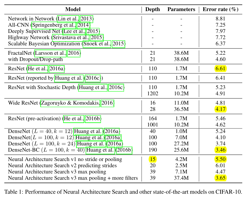
First, if we ask the controller to not predict stride or pooling, it can design a 15-layer architecture that achieves 5.50% error rate on the test set.
不预测stride（stride fix to1）和pooling的15层卷积网络，err rate：5.50

This architecture has a good balance between accuracy and depth. In fact, it is the shallowest and perhaps the most inexpensive architecture among the top performing networks in this table.
该网络的优点：深度最浅，计算量最小

This architecture is shown in Appendix A, Figure 7.

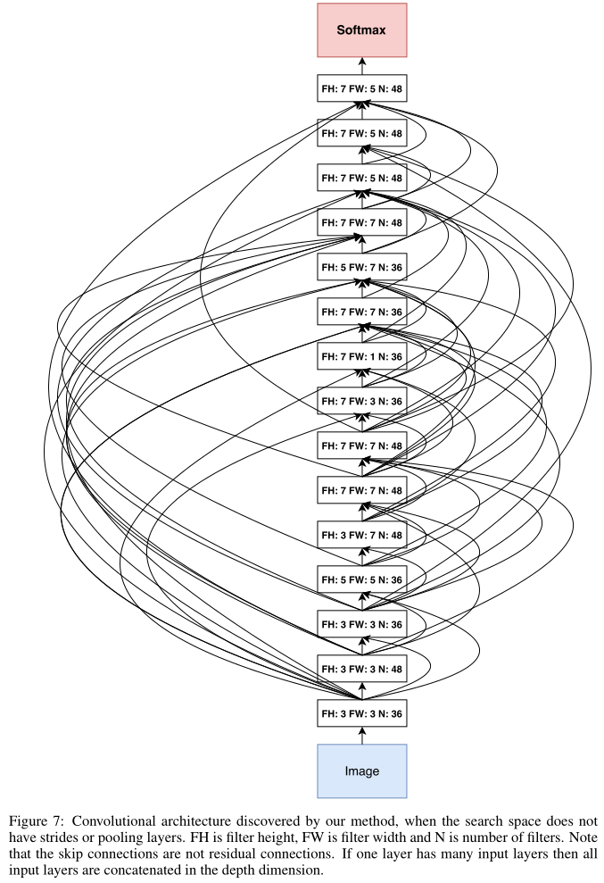
A notable feature of this architecture is that it has many rectangular filters and it prefers larger filters at the top layers. Like residual networks (He et al., 2016a), the architecture also has many one-step skip connections.
观察该结构，1.有很多矩形卷积核（⭐️ ​矩形卷积核？）2.越深的层偏爱大卷积核 3.有很多skip connections

This architecture is a local optimum in the sense that if we perturb it, its performance becomes worse.
该结构只是局部最优，对结构参数（字符串）进行微小扰动的话，会降低网络表现

In the second set of experiments, we ask the controller to predict strides in addition to other hyperparameters.
另一组实验，（stride in [1 2 3]）
In this case, it finds a 20-layer architecture that achieves 6.01% error rate on the test set, which is not much worse than the first set of experiments.
找到一个20层的结构，err rate：6.01，比第一组实验还差
Finally, if we allow the controller to include 2 pooling layers at layer 13 and layer 24 of the architectures, the controller can design a 39-layer network that achieves 4.47% which is very close to the best human-invented architecture that achieves 3.74%.
允许引入2个pooling层（分别在第13和24层），设计39层的网络，err rate：4.47

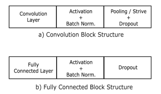
To limit the search space complexity we have our model predict 13 layers where each layer prediction is a fully connected block of 3 layers.

Additionally, we change the number of filters our model can predict from [24, 36, 48, 64] to [6, 12, 24, 36].
Our result can be improved to 3.65% by adding 40 more filters to each layer of our architecture.
Additionally this model with 40 filters added is 1.05x as fast as the DenseNet model that achieves 3.74%, while having better performance.
The DenseNet model that achieves 3.46% error rate (Huang et al., 2016b) uses 1x1 convolutions to reduce its total number of parameters, which we did not do, so it is not an exact comparison.

Conclusion

Appendix

Angular module 的 forRoot 和 forChild 方法

代码：

export class OutletModule {
  static forRoot(): ModuleWithProviders<OutletModule> {
    return {
      ngModule: OutletModule,
      providers: [
        {
          provide: APP_INITIALIZER,
          useFactory: registerOutletsFactory,
          deps: [
            [new Optional(), PROVIDE_OUTLET_OPTIONS],
            ComponentFactoryResolver,
            OutletService,
          ],
          multi: true,
        },
      ],
    };
  }

  static forChild(): ModuleWithProviders<OutletModule> {
    return {
      ngModule: OutletModule,
      providers: [
        {
          provide: MODULE_INITIALIZER,
          useFactory: registerOutletsFactory,
          deps: [
            [new Optional(), PROVIDE_OUTLET_OPTIONS],
            ComponentFactoryResolver,
            OutletService,
          ],
          multi: true,
        },
      ],
    };
  }

在详细解析这段 Angular 代码之前，让我们首先理解几个关键的 Angular 概念，包括模块（Modules）、服务提供者（Providers）、工厂函数（Factory functions）、以及模块与服务初始化器（APP_INITIALIZER 和 MODULE_INITIALIZER）。理解这些概念对深入掌握 Angular 框架至关重要。通过这段代码，我们将深入探讨 OutletModule 类如何利用 Angular 强大的依赖注入系统来配置和提供服务，特别是在应用程序初始化阶段如何动态注册路由出口（outlets）。

OutletModule 类的作用

OutletModule 是一个 Angular 模块，它提供了一个静态方法 forRoot 和一个 forChild，用于在 Angular 应用的不同层级中导入此模块。在多级路由应用中，这种模式非常有用，因为它允许模块以不同的配置被根模块和子模块所使用。通过这种方式，OutletModule 可以根据应用的结构和需要灵活地提供服务和配置。

forRoot 方法

forRoot 方法返回一个对象，该对象指定了 ngModule 和 providers。在这里，ngModule 是 OutletModule 自身，这意味着当调用 forRoot 方法时，OutletModule 将被注册到 Angular 的依赖注入框架中。

providers 数组中的配置是此模块的核心。它通过 APP_INITIALIZER 令牌提供了一个初始化函数。APP_INITIALIZER 是一个 Angular 令牌，用于注册一个或多个在应用启动时运行的初始化函数。这些函数可以是异步的，并且应用不会完成启动，直到所有通过 APP_INITIALIZER 注册的函数都运行完毕。

useFactory 指向了 registerOutletsFactory 工厂函数，这是实际注册路由出口（outlets）的地方。工厂函数的依赖（deps）包括可选的 PROVIDE_OUTLET_OPTIONS、ComponentFactoryResolver 和 OutletService。这些依赖通过 Angular 的依赖注入（DI）系统注入到工厂函数中。

• PROVIDE_OUTLET_OPTIONS 是一个可选依赖，用于传递配置选项。这里的 new Optional() 表明如果没有提供此依赖，则不会导致错误。
• ComponentFactoryResolver 用于动态加载组件。
• OutletService 可能是一个用于管理路由出口（outlets）的服务。

forChild 方法

forChild 方法的结构与 forRoot 非常相似，但它使用的是 MODULE_INITIALIZER 而不是 APP_INITIALIZER。这表明通过 forChild 方法注册的服务和配置是为了在模块级别而不是应用级别进行初始化。这对于惰性加载的模块或需要特定初始化逻辑的功能模块尤其有用。

深入 registerOutletsFactory 工厂函数

尽管代码中没有提供 registerOutletsFactory 函数的实现细节，我们可以推测其作用是利用依赖注入的 PROVIDE_OUTLET_OPTIONS、ComponentFactoryResolver 和 OutletService 来动态注册路由出口。这可能包括配置路由、注册动态加载的组件或者其他与路由出口相关的初始化任务。

结论

通过 OutletModule 的设计，我们看到了 Angular 框架灵活而强大的一面，尤其是在模块化设计、依赖注入和应用初始化方面。forRoot 和 forChild 方法提供了一种优雅的方式来根据应用的结构和初始化需求定制模块的行为。此外，使用 APP_INITIALIZER 和 MODULE_INITIALIZER 为应用及其模块提供初始化逻辑的能力展示了 Angular 在构建大型、可维护和高效的前端应用方面的优势。

ArcGIS for Windows Mobile 3.1发布

        ArcGIS WindowsMobile 3.1已经发布，正式用户可登陆Esri Customer Care Portal下载该版本。3.1在3.0版本的基础上做了少许增强和改进，但最大的改变是Esri和Trimble公司合作，共同推出了一个新的解决方案：Trimble®Positions™ Software Suite ，该解决方案专用于野外数据的采集，是一个齐全的，即拿即用的外业数据采集方案，典型特点有：

 ·支持高精度的GNSS移动数据采集；

·支持实时的（real-time）和非实时（post-processing）数据采集流程。

可从网站Technical Support tab下载到有关该解决方案的说明文档。

TrimblePosition Software Suite

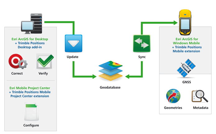
         Trimble Positions解决方案需要ArcGISfor Windows Mobile 3.1和ArcGIS for Desktop 10.1，请确认您升级到了最新版本。

显著的改进如下：

·在Windows平台上直接集成了相机；

·面积测量时支持单位“亩”；

·改进了在Windows Mobile系统上使用相机时内存的管理。

原文链接： http://blog.csdn.net/arcgis_all/article/details/8232807

Creating a Connection Between Enterprise Search and SAP HANA for ABAP CDS-Based Search Models

from SAP help

If you want to use Enterprise Search in applications that use ABAP CDS-based search models, you first have to create the connection between the ABAP system of Enterprise Search and SAP HANA. Compared to the standard configuration, there are various points you need to consider.

Prerequisites

You have installed SAP HANA in revision 102 or higher.

Process

Log on to the SAP NetWeaver system and launch the Implementation Guide (IMG) by using transaction SPRO. Navigate to the node Search and Operational Analytics Common Settings for Operational Analytics and Enterprise Search Configure Indexing Define TREX/BWA Destination or SAP HANA Database Connection . When you launch the Customizing activity, the ABAP program ESH_ADM_SET_TREX_DESTINATION starts.

If you are performing the initial configuration of the Enterprise Search system, choose Use Primary DB Connection of SAP HANA: STANDARD and then Execute.

Note

If you are using an existing Enterprise Search system that is already configured, do not change the selected database connection.
Switch to SAP HANA studio.
To assign the required authorizations to the SAP HANA users, execute the following SQL statements as the SAP HANA system user:
If you are performing the initial configuration of the Enterprise Search system, execute the following SQL statements:

GRANT EXECUTE ON SYS.ESH_CONFIG TO <SAP HANA Primary DB Connection User>;
GRANT EXECUTE ON SYS.ESH_SEARCH TO <SAP HANA Primary DB Connection User>;
GRANT SELECT ON _SYS_RT.ESH_MODEL TO <SAP HANA Primary DB Connection User>;
GRANT SELECT ON _SYS_RT.ESH_MODEL_PROPERTY TO <SAP HANA Primary DB Connection User>;
GRANT EXECUTE ON SYS.TREXVIADBSL TO <SAP HANA Primary DB Connection User>;
GRANT EXECUTE ON SYS.TREXVIADBSLWITHPARAMETER TO <SAP HANA Primary DB Connection User>;

Note

You can find the name of the user of the primary database connection (SAP HANA Primary DB Connection User) in the ABAP system in the menu System Status... in the area Database Data in the field Owner.
If you are using an existing Enterprise Search system that is already configured, execute the following SQL statements instead:

GRANT EXECUTE ON SYS.ESH_CONFIG TO <SAP HANA Primary DB Connection User>;
GRANT EXECUTE ON SYS.ESH_SEARCH TO <SAP HANA Primary DB Connection User>;
GRANT SELECT ON _SYS_RT.ESH_MODEL TO <SAP HANA Primary DB Connection User>;
GRANT EXECUTE ON SYS.TREXVIADBSL TO <SAP HANA Search User>;
GRANT EXECUTE ON SYS.TREXVIADBSLWITHPARAMETER TO <SAP HANA Search User>;

Note

You can find the name of the user of the database connection for the search (SAP HANA Search User) in the ABAP system: Start the program ESH_ADM_SET_TREX_DESTINATION and check whether the primary or secondary database connection is used. If the primary database connection is selected, use the user name of the primary database connection as the name of the user of the database connection for the search (SAP HANA Search User).

If the secondary database connection is selected, the name of the database connection is displayed in the relevant field (DB Connection Name). Start transaction DBCO to find the user name that is assigned to this database connection. This user name corresponds to the user of the database connection for the search (SAP HANA Search User).
If you are using the secondary database connection in an existing Enterprise Search system that has already been configured (see the setting under ESH_ADM_SET_TREX_DESTINATION), you must grant authorization to the user of the database connection for the search (SAP HANA Search User) to execute the SQL statement SELECT on the database schema (SAPSID) of the primary database connection.
GRANT SELECT ON SCHEMA TO ;

本文同步分享在 博客 “汪子熙”（CSDN）。
如有侵权，请联系 support@oschina.cn 删除。
本文参与 “OSC 源创计划”，欢迎正在阅读的你也加入，一起分享。

关于Searching for MobileNetV3的问题就给大家分享到这里，感谢你花时间阅读本站内容，更多关于2017-ICLR-Neural Architecture Search with Reinforcement Learning 论文阅读、Angular module 的 forRoot 和 forChild 方法、ArcGIS for Windows Mobile 3.1发布、Creating a Connection Between Enterprise Search and SAP HANA for ABAP CDS-Based Search Models等相关知识的信息别忘了在本站进行查找喔。

本文标签：

• Searching_for_MobileNetV3
• MobileNet_V3
• Deep_Learning_Models
• Computer_Vision