对于想了解KibanaTimelion插件如何在elasticsearch中指定字段的读者,本文将是一篇不可错过的文章,我们将详细介绍elasticsearchkibana配置,并且为您提供关于Bui
对于想了解Kibana Timelion插件如何在elasticsearch中指定字段的读者,本文将是一篇不可错过的文章,我们将详细介绍elasticsearch kibana配置,并且为您提供关于Building real-time dashboard applications with Apache Flink, Elasticsearch, and Kibana、docker+springboot+elasticsearch+kibana+elasticsearch-head整合(详细说明 ,看这一篇就够了)、elasticsearch + kibana、Elasticsearch + Kibana 安装的有价值信息。
本文目录一览:- Kibana Timelion插件如何在elasticsearch中指定字段(elasticsearch kibana配置)
- Building real-time dashboard applications with Apache Flink, Elasticsearch, and Kibana
- docker+springboot+elasticsearch+kibana+elasticsearch-head整合(详细说明 ,看这一篇就够了)
- elasticsearch + kibana
- Elasticsearch + Kibana 安装
")
Kibana Timelion插件如何在elasticsearch中指定字段(elasticsearch kibana配置)
我正在尝试将Timelion插件用于kibana。
我在elasticsearch中有一个数据集,其结构可能是这样的:
{ "_index": "metrics-2016-03", "_type": "gauge", "_id": "AVM2O7gbLYPaOnNTBgG0", "_score": 1, "_source": { "name": "kafka.network.RequestChannel.ResponseQueueSize", "@timestamp": "2016-03-02T07:29:56.000+0000", "value": 4, "host": "localhost" }}我想将"value"字段显示为y轴和"@timestamp"x轴,该怎么办?
我尝试了该.es()功能,但此功能似乎将计数设置为默认值,而不是数据源中的“值”字段。
答案1
小编典典Timelion将预定义的时间间隔用于其时间图。为了绘制“值”作为时间的函数,您可以将粒度设置为“自动”并使用以下字符串:
.es(metric=''max:value'')您也可以将粒度设置为最小,然后添加.fit(carry)到上述字符串中以填充空值,在这种情况下,您可以max用min或替换avg,它将产生相同的图(sum此处不起作用)。

Building real-time dashboard applications with Apache Flink, Elasticsearch, and Kibana
https://www.elastic.co/cn/blog/building-real-time-dashboard-applications-with-apache-flink-elasticsearch-and-kibana
Fabian Hueske
Share
Gaining actionable insights from continuously produced data in real-time is a common requirement for many businesses today. A wide-spread use case for real-time data processing is dashboarding. A typical architecture to support such a use case is based on a data stream processor, a data store with low latency read/write access, and a visualization framework.
In this blog post, we demonstrate how to build a real-time dashboard solution for stream data analytics using Apache Flink, Elasticsearch, and Kibana. The following figure depicts our system architecture.
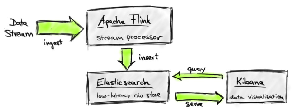
In our architecture, Apache Flink executes stream analysis jobs that ingest a data stream, apply transformations to analyze, transform, and model the data in motion, and write their results to an Elasticsearch index. Kibana connects to the index and queries it for data to visualize. All components of our architecture are open source systems under the Apache License 2.0. We show how to implement a Flink DataStream program that analyzes a stream of taxi ride events and writes its results to Elasticsearch and give instructions on how to connect and configure Kibana to visualize the analyzed data in real-time.
Why use Apache Flink for stream processing?
Before we dive into the details of implementing our demo application, we discuss some of the features that make Apache Flink an outstanding stream processor. Apache Flink 0.10, which was recently released, comes with a competitive set of stream processing features, some of which are unique in the open source domain. The most important ones are:
- Support for event time and out of order streams: In reality, streams of events rarely arrive in the order that they are produced, especially streams from distributed systems and devices. Until now, it was up to the application programmer to correct this “time drift”, or simply ignore it and accept inaccurate results, as streaming systems (at least in the open source world) had no support for event time (i.e., processing events by the time they happened in the real world). Flink 0.10 is the first open source engine that supports out of order streams and which is able to consistently process events according to their timestamps.
- Expressive and easy-to-use APIs in Scala and Java: Flink''s DataStream API ports many operators which are well known from batch processing APIs such as map, reduce, and join to the streaming world. In addition, it provides stream-specific operations such as window, split, and connect. First-class support for user-defined functions eases the implementation of custom application behavior. The DataStream API is available in Scala and Java.
- Support for sessions and unaligned windows: Most streaming systems have some concept of windowing, i.e., a grouping of events based on some function of time. Unfortunately, in many systems these windows are hard-coded and connected with the system’s internal checkpointing mechanism. Flink is the first open source streaming engine that completely decouples windowing from fault tolerance, allowing for richer forms of windows, such as sessions.
- Consistency, fault tolerance, and high availability: Flink guarantees consistent state updates in the presence of failures (often called “exactly-once processing”), and consistent data movement between selected sources and sinks (e.g., consistent data movement between Kafka and HDFS). Flink also supports worker and master failover, eliminating any single point of failure.
- Low latency and high throughput: We have clocked Flink at 1.5 million events per second per core, and have also observed latencies in the 25 millisecond range for jobs that include network data shuffling. Using a tuning knob, Flink users can navigate the latency-throughput trade off, making the system suitable for both high-throughput data ingestion and transformations, as well as ultra low latency (millisecond range) applications.
- Connectors and integration points: Flink integrates with a wide variety of open source systems for data input and output (e.g., HDFS, Kafka, Elasticsearch, HBase, and others), deployment (e.g., YARN), as well as acting as an execution engine for other frameworks (e.g., Cascading, Google Cloud Dataflow). The Flink project itself comes bundled with a Hadoop MapReduce compatibility layer, a Storm compatibility layer, as well as libraries for machine learning and graph processing.
- Developer productivity and operational simplicity: Flink runs in a variety of environments. Local execution within an IDE significantly eases development and debugging of Flink applications. In distributed setups, Flink runs at massive scale-out. The YARN mode allows users to bring up Flink clusters in a matter of seconds. Flink serves monitoring metrics of jobs and the system as a whole via a well-defined REST interface. A build-in web dashboard displays these metrics and makes monitoring of Flink very convenient.
The combination of these features makes Apache Flink a unique choice for many stream processing applications.
Building a demo application with Flink, Elasticsearch, and Kibana
Our demo ingests a stream of taxi ride events and identifies places that are popular within a certain period of time, i.e., we compute every 5 minutes the number of passengers that arrived at each location within the last 15 minutes by taxi. This kind of computation is known as a sliding window operation. We share a Scala implementation of this application (among others) on Github. You can easily run the application from your IDE by cloning the repository and importing the code. The repository''s README file provides more detailed instructions.
Analyze the taxi ride event stream with Apache Flink
For the demo application, we generate a stream of taxi ride events from a public dataset of the New York City Taxi and LimousineCommission (TLC). The data set consists of records about taxi trips in New York City from 2009 to 2015. We took some of this data and converted it into a data set of taxi ride events by splitting each trip record into a ride start and a ride end event. The events have the following schema:
rideId: Long time: DateTime // start or end time isStart: Boolean // true = ride start, false = ride end location: GeoPoint // lon/lat of pick-up or drop-off location passengerCnt: short travelDist: float // -1 on start events
We implemented a custom SourceFunction to serve a DataStream[TaxiRide] from the ride event data set. In order to generate the stream as realistically as possible, events are emitted by their timestamps. Two events that occurred ten minutes after each other in reality are ingested by Flink with a ten minute lag. A speed-up factor can be specified to “fast-forward” the stream, i.e., with a speed-up factor of 2.0, these events are served five minutes apart. Moreover, the source function adds a configurable random delay to each event to simulate the real-world jitter. Given this stream of taxi ride events, our task is to compute every five minutes the number of passengers that arrived within the last 15 minutes at locations in New York City by taxi.
As a first step we obtain a StreamExecutionEnvironment and set the TimeCharacteristic to EventTime. Event time mode guarantees consistent results even in case of historic data or data which is delivered out-of-order.
val env = StreamExecutionEnvironment.getExecutionEnvironment env.setStreamTimeCharacteristic(TimeCharacteristic.EventTime)
Next, we define the data source that generates a DataStream[TaxiRide] with at most 60 seconds serving delay (events are out of order by max. 1 minute) and a speed-up factor of 600 (10 minutes are served in 1 second).
// Define the data source
val rides: DataStream[TaxiRide] = env.addSource(new TaxiRideSource( “./data/nycTaxiData.gz”, 60, 600.0f))
Since we are only interested in locations that people travel to (and not where they come from) and because the original data is a little bit messy (locations are not always correctly specified), we apply a few filters to first cleanse the data.
val cleansedRides = rides
 // filter for ride end events .filter( !_.isStart ) // filter for events in NYC .filter( r => NycGeoUtils.isInNYC(r.location) )
The location of a taxi ride event is defined as a pair of continuous longitude/latitude values. We need to map them into a finite set of regions in order to be able to aggregate events by location. We do this by defining a grid of approx. 100x100 meter cells on the area of New York City. We use a utility function to map event locations to cell ids and extract the passenger count as follows:
// map location coordinates to cell Id, timestamp, and passenger count
val cellIds: DataStream[(Int, Long, Short)] = cleansedRides .map { r => ( NycGeoUtils.mapToGridCell(r.location), r.time.getMillis, r.passengerCnt ) }
After these preparation steps, we have the data that we would like to aggregate. Since we want to compute the passenger count for each location (cell id), we start by keying (partitioning by key) the stream by cell id (_._1). Subsequently, we define a sliding time window and run a <code>WindowFunction</code>; by calling apply():
val passengerCnts: DataStream[(Int, Long, Int)] = cellIds // key stream by cell Id .keyBy(_._1) // define sliding window on keyed stream .timeWindow(Time.minutes(15), Time.minutes(5)) // count events in window .apply { ( cell: Int, window: TimeWindow, events: Iterable[(Int, Short)], out: Collector[(Int, Long, Int)]) => out.collect( ( cell, window.getEnd, events.map( _._2 ).sum ) ) }
The timeWindow() operation groups stream events into finite sets of records on which a window or aggregation function can be applied. For our application, we call apply() to process the windows using a WindowFunction. The WindowFunction receives four parameters, a Tuple that contains the key of the window, a Window object that contains details such as the start and end time of the window, an Iterable over all elements in the window, and a Collector to collect the records emitted by the WindowFunction. We want to count the number of passengers that arrive within the window’s time bounds. Therefore, we have to emit a single record that contains the grid cell id, the end time of the window, and the sum of the passenger counts which is computed by extracting the individual passenger counts from the iterable (events.map( _._2)) and summing them (.sum).
Finally, we translate the cell id back into a GeoPoint (referring to the center of the cell) and print the result stream to the standard output. The final env.execute() call takes care of submitting the program for execution.
val cntByLocation: DataStream[(Int, Long, GeoPoint, Int)] = passengerCnts // map cell Id back to GeoPoint .map( r => (r._1, r._2, NycGeoUtils.getGridCellCenter(r._1), r._3 ) ) cntByLocation // print to console .print() env.execute(“Total passenger count per location”)
If you followed the instructions to import the demo code into your IDE, you can run theSlidingArrivalCount.scala program by executing its main() methods. You will see Flink’s log messages and the computed results being printed to the standard output.
You might wonder why the the program produces results much faster than once every five minutes per location. This is due to the event time processing mode. Since all time-based operations (such as windows) are based on the timestamps of the events, the program becomes independent of the speed at which the data is served. This also means that you can process historic data which is read at full speed from some data store and data which is continuously produced with exactly the same program.
Our streaming program will run for a few minutes until the packaged data set is completely processed but you can terminate it at any time. As a next step, we show how to write the result stream into an Elasticsearch index.
Prepare the Elasticsearch
The Flink Elasticsearch connector depends on Elasticsearch 1.7.3. Follow these steps to setup Elasticsearch and to create an index.
- Download Elasticsearch 1.7.3 as .tar (or .zip) archive here.
- Extract the archive file:
tar xvfz elasticsearch-1.7.3.tar.gz - Enter the extracted directory and start Elasticsearch
cd elasticsearch-1.7.3 ./bin/elasticsearch - Create an index called “nyc-idx”:
curl -XPUT "http://localhost:9200/nyc-idx" - Create an index mapping called “popular-locations”:
curl -XPUT "http://localhost:9200/nyc-idx/_mapping/popular-locations" -d'' { "popular-locations" : { "properties" : { "cnt": {"type": "integer"}, "location": {"type": "geo_point"}, "time": {"type": "date"} } } }''
The SlidingArrivalCount.scala program is prepared to write data to the Elasticsearch index you just created but requires a few parameters to be set at the beginning of the main() function. Please set the parameters as follows:
val writeToElasticsearch = true val elasticsearchHost = // look up the IP address in the Elasticsearch logs val elasticsearchPort = 9300
Now, everything is set up to fill our index with data. When you run the program by executing the main() method again, the program will write the resulting stream to the standard output as before but also insert the records into the nyc-idx Elasticsearch index.
If you later want to clear the nyc-idx index, you can simply drop the mapping by running
curl -XDELETE ''http://localhost:9200/nyc-idx/popular-locations''and create the mapping again with the previous command.
Visualizing the results with Kibana
In order to visualize the data that is inserted into Elasticsearch, we install Kibana 4.1.3 which is compatible with Elasticsearch 1.7.3. The setup is basically the same as for Elasticsearch.
1. Download Kibana 4.1.3 for your environment here.
2. Extract the archive file.
3. Enter the extracted folder and start Kibana by running the start script: ./bin/kibana
4. Open http://localhost:5601 in your browser to access Kibana.
Next we need to configure an index pattern. Enter the index name “nyc-idx” and click on “Create”. Do not uncheck the “Index contains time-based events” option. Now, Kibana knows about our index and we can start to visualize our data.
First click on the “Discover” button at the top of the page. You will find that Kibana tells you “No results found”.
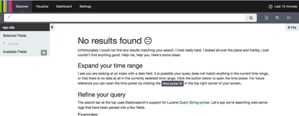
This is because Kibana restricts time-based events by default to the last 15 minutes. Since our taxi ride data stream starts on January, 1st 2013, we need to adapt the time range that is considered by Kibana. This is done by clicking on the label “Last 15 Minutes” in the top right corner and entering an absolute time range starting at 2013-01-01 and ending at 2013-01-06.
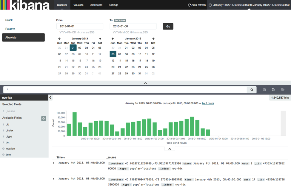
We have told Kibana where our data is and the valid time range and can continue to visualize the data. For example we can visualize the arrival counts on a map. Click on the “Visualize” button at the top of the page, select “Tile map”, and click on “From a new search”.
See the following screenshot for the tile map configuration (left-hand side).
Another interesting visualization is to plot the number of arriving passengers over time. Click on “Visualize” at the top, select “Vertical bar chart”, and select “From a new search”. Again, have a look at the following screenshot for an example for how to configure the chart.
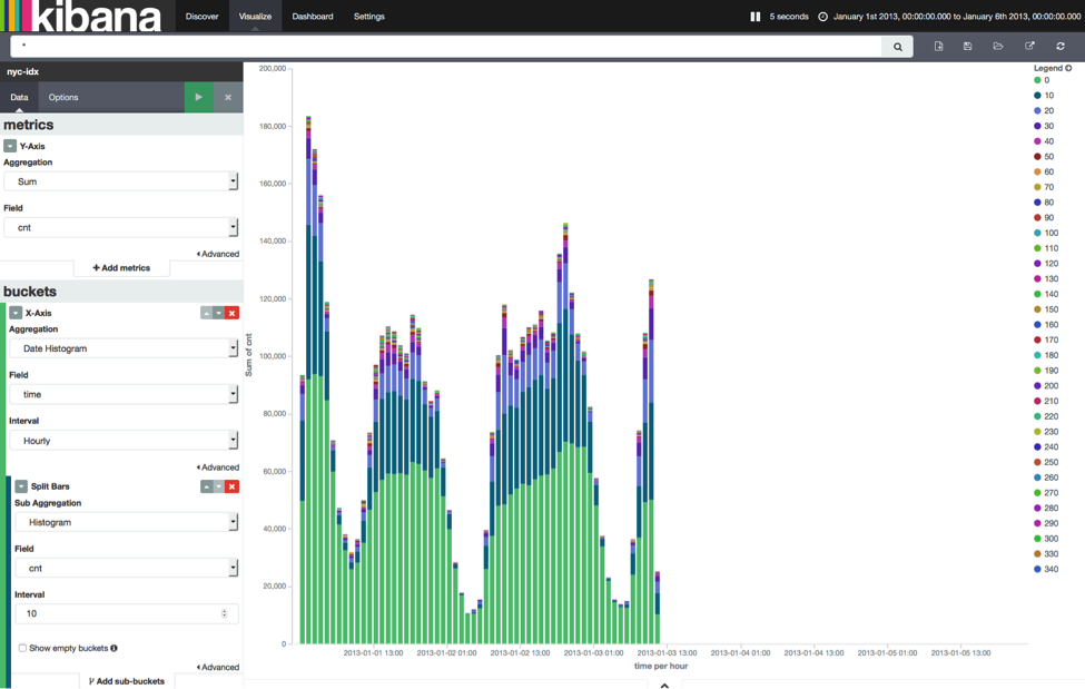
Kibana offers many more chart types and visualization options which are out of the scope of this post. You can easily play around with this setup, explore Kibana’s features, and implement your own Flink DataStream programs to analyze taxi rides in New York City.
We’re done and hope you had some fun
In this blog post we demonstrated how to build a real-time dashboard application with Apache Flink, Elasticsearch, and Kibana. By supporting event-time processing, Apache Flink is able to produce meaningful and consistent results even for historic data or in environments where events arrive out-of-order. The expressive DataStream API with flexible window semantics results in significantly less custom application logic compared to other open source stream processing solutions. Finally, connecting Flink with Elasticsearch and visualizing the real-time data with Kibana is just a matter of a few minutes. We hope you enjoyed running our demo application and had fun playing around with the code.
Fabian Hueske is a PMC member of Apache Flink. He is contributing to Flink  since its earliest days when it started as research project as part of his PhD studies at TU Berlin. Fabian did internships with IBM Research, SAP Research, and Microsoft Research and is a co-founder of data Artisans, a Berlin-based start-up devoted to foster Apache Flink. He is interested in distributed data processing and query optimization.
")
docker+springboot+elasticsearch+kibana+elasticsearch-head整合(详细说明 ,看这一篇就够了)
一开始是没有打算写这一篇博客的,但是看见好多朋友问关于elasticsearch的坑,决定还是写一份详细的安装说明与简单的测试demo,只要大家跟着我的步骤一步步来,100%是可以测试成功的。
一. docker安装
本人使用的是centos6,安装命令如下:
1.首先使用epel库安装docker
yum install -y http://mirrors.yun-idc.com/epel/6/i386/epel-release-6-8.noarch.rpm
yum install -y docker-io
安装完成后,使用命令 service docker start 启动docker
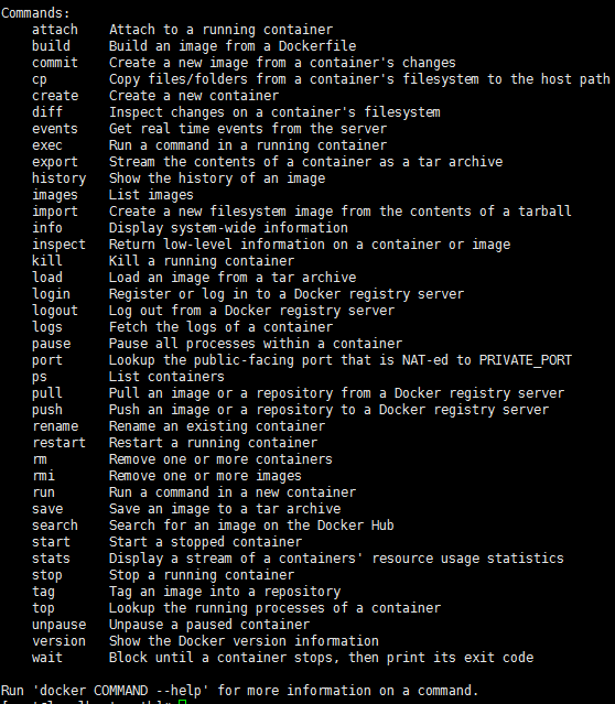
控制台输入docker ,出现如下界面表示安装成功

如果提示检查软件失败什么的,是因为之前先装了docker,再装了docker-io,直接使用命令 yum remove docker 删除docker,再执行
yum install -y docker-io 即可。
如果仍然提示 no package avalible...
使用rpm安装docker:
rpm -ivh docker源的方式 yum install
Ubuntu/Debian: curl -sSL https://get.docker.com | sh
Linux 64bit binary: https://get.docker.com/builds/Linux/x86_64/docker-1.7.1
Darwin/OSX 64bit client binary: https://get.docker.com/builds/Darwin/x86_64/docker-1.7.1
Darwin/OSX 32bit client binary: https://get.docker.com/builds/Darwin/i386/docker-1.7.1
Linux 64bit tgz: https://get.docker.com/builds/Linux/x86_64/docker-1.7.1.tgz
Windows 64bit client binary: https://get.docker.com/builds/Windows/x86_64/docker-1.7.1.exe
Windows 32bit client binary: https://get.docker.com/builds/Windows/i386/docker-1.7.1.exe
Centos 6/RHEL 6: https://get.docker.com/rpm/1.7.1/centos-6/RPMS/x86_64/docker-engine-1.7.1-1.el6.x86_64.rpm
https://get.docker.com/rpm/1.7.1/centos-6/RPMS/x86_64/docker-engine-1.7.1-1.el6.x86_64.rpm
Centos 7/RHEL 7: https://get.docker.com/rpm/1.7.1/centos-7/RPMS/x86_64/docker-engine-1.7.1-1.el7.centos.x86_64.rpm
Fedora 20: https://get.docker.com/rpm/1.7.1/fedora-20/RPMS/x86_64/docker-engine-1.7.1-1.fc20.x86_64.rpm
Fedora 21: https://get.docker.com/rpm/1.7.1/fedora-21/RPMS/x86_64/docker-engine-1.7.1-1.fc21.x86_64.rpm
Fedora 22: https://get.docker.com/rpm/1.7.1/fedora-22/RPMS/x86_64/docker-engine-1.7.1-1.fc22.x86_64.rpm
2.下载elasticsearch 镜像
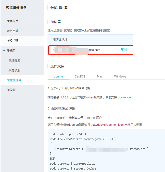
在下载elasticsearch镜像之前,可以先改一下docker的镜像加速功能,我是用的阿里云的镜像加速,登录阿里云官网,产品-->云计算基础-->容器镜像服务, 进入管理控制台,如下图所示,复制加速器地址。
进入虚拟机,vim /etc/sysconfig/docker,加入下面一行配置
other_args="--registry-mirror=https://xxxx.aliyuncs.com"
:wq 保存退出
service docker restart 重启docker服务
ps -aux|grep docker 输入如下命令查看docker信息,出现如下信息则加速器配置成功
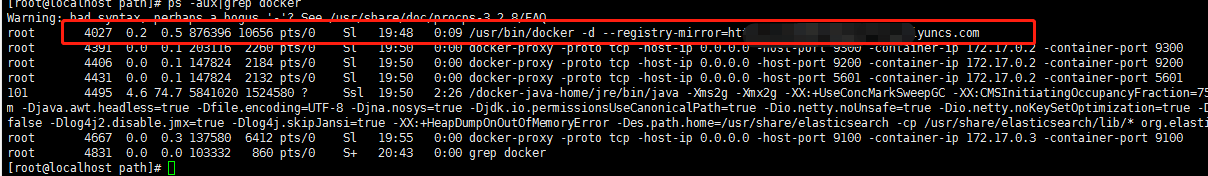
然后就可以快速pull镜像了。
docker pull elasticsearch
docker pull kibana
docker pull mobz/elasticsearch-head:5
将我们需要的三个镜像拉取下来
mkdir -p /opt/elasticsearch/data
vim /opt/elasticsearch/elasticsearch.yml


docker run --name elasticsearch -p 9200:9200 -p 9300:9300 -p 5601:5601 -e "discovery.type=single-node" -v /opt/elasticsearch/elasticsearch.yml:/usr/share/elasticsearch/config/elasticsearch.yml -v /opt/elasticsearch/data:/usr/share/elasticsearch/data -d elasticsearch
elasticsearch.yml 配置文件内容:
cluster.name: elasticsearch_cluster
node.name: node-master
node.master: true
node.data: true
http.port: 9200
network.host: 0.0.0.0
network.publish_host: 192.168.6.77
discovery.zen.ping.unicast.hosts: ["192.168.6.77","192.168.6.78"]
http.host: 0.0.0.0
http.cors.enabled: true
http.cors.allow-origin: "*"
bootstrap.memory_lock: false
bootstrap.system_call_filter: false
# Uncomment the following lines for a production cluster deployment
#transport.host: 0.0.0.0
discovery.zen.minimum_master_nodes: 1
注意我的elasticsearch 是在两台服务器上的,所以集群部署的时候可以省略端口号,因为都是9300,如果你的集群是部署在同一台os上,则需要区分出来端口号。
cluster.name: elasticsearch_cluster 集群名字,所有集群统一。
node.name: node-master 你的节点名称,所有集群必须区分开。
http.cors.enabled: true
http.cors.allow-origin: "*"  支持跨域
discovery.zen.minimum_master_nodes: 1 可被发现作为主节点的数量
network.publish_host: 192.168.6.77 对外公布服务的真实IP
network.host: 0.0.0.0 开发环境可以设置成0.0.0.0,真正的生产环境需要指定IP地址。
我们启动elasticsearch容器多加了一个端口映射 -p 5601:5601 目的是让kibana使用该容器的端口映射,无需指定kibana容器的映射了。
启动kibana:
docker run --name kibana -e ELASTICSEARCH_URL=http://127.0.0.1:9200 --net=container:elasticsearch -d kibana--net=container:elasticsearch 命令为指定使用elasticsearch的映射
这个时候,一般elasticsearch是启动报错的,我们需要修改一下linux的文件配置,如文件描述符的大小等。
需要修改的文件一共两个:
切换到root用户
1、vi /etc/security/limits.conf 修改如下配置
* soft nofile 65536
* hard nofile 131072

2、vi /etc/sysctl.conf 添加配置
vm.max_map_count=655360
运行命令 sysctl -p
这个时候配置完了输入命令
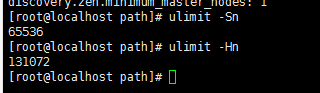
ulimit -Sn
ulimit -Hn
出现如下信息即配置成功。
可是这个时候重启容器依然是报错的,没报错是你运气好,解决办法是重启一下docker就OK了。
service docker restart
然后重启elasticsearch 容器
docker restart elasticsearch
访问ip:9200
出现如下信息,则elasticsearch 启动成功
{
  "name" : "node-master",
  "cluster_name" : "elasticsearch_cluster",
  "cluster_uuid" : "QzD1rYUOSqmpoXPYQqolqQ",
  "version" : {
    "number" : "5.6.12",
    "build_hash" : "cfe3d9f",
    "build_date" : "2018-09-10T20:12:43.732Z",
    "build_snapshot" : false,
    "lucene_version" : "6.6.1"
  },
  "tagline" : "You Know, for Search"
}
接着同样的操作,在另外一台os上启动elasticsearch,两台不同的地方一是第二台我们不需要做-p 5601:5601的端口映射,第二是elasticsearch.yml配置文件的一些不同:
cluster.name: elasticsearch_cluster
node.name: node-slave
node.master: false
node.data: true
http.port: 9200
network.host: 0.0.0.0
network.publish_host: 192.168.6.78
discovery.zen.ping.unicast.hosts: ["192.168.6.77:9300","192.168.6.78:9300"]
http.host: 0.0.0.0
http.cors.enabled: true
http.cors.allow-origin: "*"
bootstrap.memory_lock: false
bootstrap.system_call_filter: false
# Uncomment the following lines for a production cluster deployment
# #transport.host: 0.0.0.0
# #discovery.zen.minimum_master_nodes: 1
#两台os中的elasticsearch都启动成功后,便可以启动kibana和head了。
重启kibana
docker restart kibana
访问http://ip:5601
出现如下页面则kibana启动成功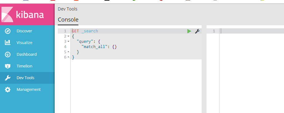
启动elasticsearch-head监控es服务
docker run -d -p 9100:9100 mobz/elasticsearch-head:5
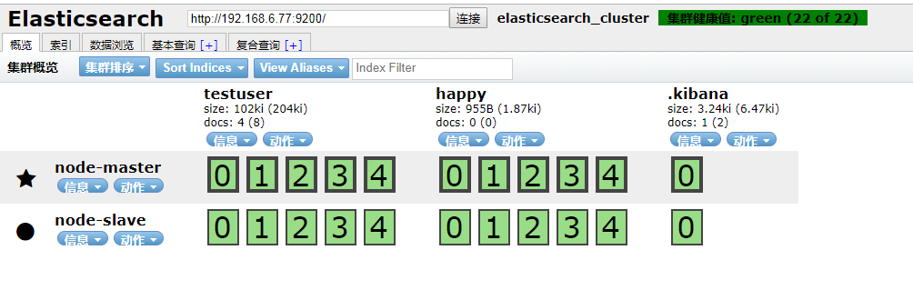
访问ip:9100
出现如下界面即启动head成功
到此我们的准备工作算是完成了,接下来新建springboot项目,pom引入
<dependency>
<groupId>org.springframework.boot</groupId>
<artifactId>spring-boot-starter-data-elasticsearch</artifactId>
</dependency>
其他mvc mybatis配置在此不再赘述,application.yml配置如下:
spring:
  data:
   elasticsearch:
    cluster-nodes: 192.168.6.77:9300
    repositories.enabled: true
    cluster-name: elasticsearch_cluster
编写仓库测试类 UserRepository:
package com.smkj.user.repository;

import org.springframework.data.elasticsearch.repository.ElasticsearchRepository;
import org.springframework.stereotype.Component;

import com.smkj.user.entity.XymApiUser;

/**
 * @author dalaoyang
 * @Description
 * @project springboot_learn
 * @package com.dalaoyang.repository
 * @email yangyang@dalaoyang.cn
 * @date 2018/5/4
 */
@Component
public interface UserRepository extends ElasticsearchRepository<XymApiUser,String> {
}
实体类中,加上如下注解:
@SuppressWarnings("serial")
@AllArgsConstructor
@NoArgsConstructor
@Data
@Accessors(chain=true)
@Document(indexName = "testuser",type = "XymApiUser")
最后一个注解是使用elasticsearch必加的,类似数据库和数据表映射
上边的几个就是贴出来给大家推荐一下lombok这个小东东,挺好用的,具体使用方法可以自行百度,不喜欢的同学可以直接删掉。
然后编写controller:
package com.smkj.user.controller;

import java.util.List;

import org.elasticsearch.action.get.GetResponse;
import org.elasticsearch.client.transport.TransportClient;
import org.elasticsearch.index.query.QueryBuilder;
import org.elasticsearch.index.query.QueryBuilders;
import org.elasticsearch.index.query.functionscore.FunctionScoreQueryBuilder;
import org.elasticsearch.index.query.functionscore.ScoreFunctionBuilders;
import org.springframework.beans.factory.annotation.Autowired;
import org.springframework.data.domain.Page;
import org.springframework.data.domain.PageRequest;
import org.springframework.data.domain.Pageable;
import org.springframework.data.elasticsearch.core.query.NativeSearchQueryBuilder;
import org.springframework.data.elasticsearch.core.query.SearchQuery;
import org.springframework.data.web.PageableDefault;
import org.springframework.http.HttpStatus;
import org.springframework.http.ResponseEntity;
import org.springframework.web.bind.annotation.GetMapping;
import org.springframework.web.bind.annotation.PathVariable;
import org.springframework.web.bind.annotation.RestController;

import com.google.common.collect.Lists;
import com.smkj.user.entity.XymApiUser;
import com.smkj.user.repository.UserRepository;
import com.smkj.user.service.UserService;

@RestController
public class UserController {
    @Autowired
    private UserService userService;
    @Autowired
    private UserRepository userRepository;
     @Autowired
        private TransportClient client;
@GetMapping("user/{id}")
    public XymApiUser getUserById(@PathVariable String id) {
    XymApiUser apiuser = userService.selectByPrimaryKey(id);
    userRepository.save(apiuser);
    System.out.println(apiuser.toString());
    return apiuser;

    }
/**
 * @param title   搜索标题
 * @param pageable page = 第几页参数, value = 每页显示条数
 */
@GetMapping("get/{id}")
public ResponseEntity  search(@PathVariable String id,@PageableDefault(page = 1, value = 10) Pageable pageable){
       if (id.isEmpty()) {
           return new ResponseEntity(HttpStatus.NOT_FOUND);
       }

    // 通过索引、类型、id向es进行查询数据
       GetResponse response = client.prepareGet("testuser", "xymApiUser", id).get();
       if (!response.isExists()) {
           return new ResponseEntity(HttpStatus.NOT_FOUND);
       }

       // 返回查询到的数据
       return new ResponseEntity(response.getSource(), HttpStatus.OK);
}


/**
 * 3、查   +++:分页、分数、分域(结果一个也不少)
 * @param page
 * @param size
 * @param q
 * @return
 * @return
 */
@GetMapping("/{page}/{size}/{q}")
public Page<XymApiUser> searchCity(@PathVariable Integer page, @PathVariable Integer size, @PathVariable String q) {

    SearchQuery searchQuery = new NativeSearchQueryBuilder()
            .withQuery( QueryBuilders.prefixQuery("cardNum",q))
            .withPageable(PageRequest.of(page, size))
            .build();
    Page<XymApiUser> pagea = userRepository.search(searchQuery);
    System.out.println(pagea.getTotalPages());
    return pagea;

}


}
访问 http://localhost:8080/0/10/6212263602070571344
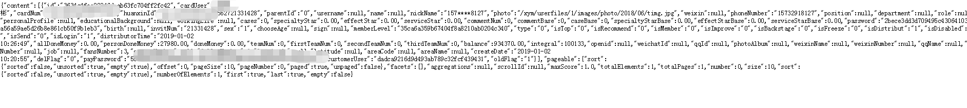
到此结束,不明白的朋友可以留言。

elasticsearch + kibana
https://www.elastic.co/cn/
全文搜索属于最常见的需求,开源的 Elasticsearch (以下简称 Elastic)是目前全文搜索引擎的首选。
它可以快速地储存、搜索和分析海量数据。维基百科、Stack Overflow、Github 都采用它。

Elastic 的底层是开源库 Lucene。但是,你没法直接用 Lucene,必须自己写代码去调用它的接口。Elastic 是 Lucene 的封装,提供了 REST API 的操作接口,开箱即用。
本文从零开始,讲解如何使用 Elastic 搭建自己的全文搜索引擎。每一步都有详细的说明,大家跟着做就能学会。
一、安装
Elastic 需要 Java 8 环境。如果你的机器还没安装 Java,可以参考这篇文章,注意要保证环境变量JAVA_HOME正确设置。
安装完 Java,就可以跟着官方文档安装 Elastic。直接下载压缩包比较简单。
$ wget https://artifacts.elastic.co/downloads/elasticsearch/elasticsearch-5.5.1.zip
$ unzip elasticsearch-5.5.1.zip
$ cd elasticsearch-5.5.1/
接着,进入解压后的目录,运行下面的命令,启动 Elastic。
$ ./bin/elasticsearch
如果这时报错"max virtual memory areas vm.maxmapcount [65530] is too low",要运行下面的命令。
$ sudo sysctl -w vm.max_map_count=262144
如果一切正常,Elastic 就会在默认的9200端口运行。这时,打开另一个命令行窗口,请求该端口,会得到说明信息。
$ curl localhost:9200

{
  "name" : "atntrTf",
  "cluster_name" : "elasticsearch",
  "cluster_uuid" : "tf9250XhQ6ee4h7YI11anA",
  "version" : {
    "number" : "5.5.1",
    "build_hash" : "19c13d0",
    "build_date" : "2017-07-18T20:44:24.823Z",
    "build_snapshot" : false,
    "lucene_version" : "6.6.0"
  },
  "tagline" : "You Know, for Search"
}
上面代码中,请求9200端口,Elastic 返回一个 JSON 对象,包含当前节点、集群、版本等信息。
按下 Ctrl + C,Elastic 就会停止运行。
默认情况下,Elastic 只允许本机访问,如果需要远程访问,可以修改 Elastic 安装目录的config/elasticsearch.yml文件,去掉network.host的注释,将它的值改成0.0.0.0,然后重新启动 Elastic。
network.host: 0.0.0.0
上面代码中,设成0.0.0.0让任何人都可以访问。线上服务不要这样设置,要设成具体的 IP。
二、基本概念
2.1 Node 与 Cluster
Elastic 本质上是一个分布式数据库,允许多台服务器协同工作,每台服务器可以运行多个 Elastic 实例。
单个 Elastic 实例称为一个节点(node)。一组节点构成一个集群(cluster)。
2.2 Index
Elastic 会索引所有字段,经过处理后写入一个反向索引(Inverted Index)。查找数据的时候,直接查找该索引。
所以,Elastic 数据管理的顶层单位就叫做 Index(索引)。它是单个数据库的同义词。每个 Index (即数据库)的名字必须是小写。
下面的命令可以查看当前节点的所有 Index。
$ curl -X GET ''http://localhost:9200/_cat/indices?v''
2.3 Document
Index 里面单条的记录称为 Document(文档)。许多条 Document 构成了一个 Index。
Document 使用 JSON 格式表示,下面是一个例子。
{
  "user": "张三",
  "title": "工程师",
  "desc": "数据库管理"
}
同一个 Index 里面的 Document,不要求有相同的结构(scheme),但是最好保持相同,这样有利于提高搜索效率。
2.4 Type
Document 可以分组,比如weather这个 Index 里面,可以按城市分组(北京和上海),也可以按气候分组(晴天和雨天)。这种分组就叫做 Type,它是虚拟的逻辑分组,用来过滤 Document。
不同的 Type 应该有相似的结构(schema),举例来说,id字段不能在这个组是字符串,在另一个组是数值。这是与关系型数据库的表的一个区别。性质完全不同的数据(比如products和logs)应该存成两个 Index,而不是一个 Index 里面的两个 Type(虽然可以做到)。
下面的命令可以列出每个 Index 所包含的 Type。
$ curl ''localhost:9200/_mapping?pretty=true''
根据规划,Elastic 6.x 版只允许每个 Index 包含一个 Type,7.x 版将会彻底移除 Type。
三、新建和删除 Index
新建 Index,可以直接向 Elastic 服务器发出 PUT 请求。下面的例子是新建一个名叫weather的 Index。
$ curl -X PUT ''localhost:9200/weather''
服务器返回一个 JSON 对象,里面的acknowledged字段表示操作成功。
{
  "acknowledged":true,
  "shards_acknowledged":true
}
然后,我们发出 DELETE 请求,删除这个 Index。
$ curl -X DELETE ''localhost:9200/weather''
四、中文分词设置
首先,安装中文分词插件。这里使用的是 ik,也可以考虑其他插件(比如 smartcn)。
$ ./bin/elasticsearch-plugin install https://github.com/medcl/elasticsearch-analysis-ik/releases/download/v5.5.1/elasticsearch-analysis-ik-5.5.1.zip
上面代码安装的是5.5.1版的插件,与 Elastic 5.5.1 配合使用。
接着,重新启动 Elastic,就会自动加载这个新安装的插件。
然后,新建一个 Index,指定需要分词的字段。这一步根据数据结构而异,下面的命令只针对本文。基本上,凡是需要搜索的中文字段,都要单独设置一下。
$ curl -X PUT ''localhost:9200/accounts'' -d ''
{
  "mappings": {
    "person": {
      "properties": {
        "user": {
          "type": "text",
          "analyzer": "ik_max_word",
          "search_analyzer": "ik_max_word"
        },
        "title": {
          "type": "text",
          "analyzer": "ik_max_word",
          "search_analyzer": "ik_max_word"
        },
        "desc": {
          "type": "text",
          "analyzer": "ik_max_word",
          "search_analyzer": "ik_max_word"
        }
      }
    }
  }
}''
上面代码中,首先新建一个名称为accounts的 Index,里面有一个名称为person的 Type。person有三个字段。
- user
- title
- desc
这三个字段都是中文,而且类型都是文本(text),所以需要指定中文分词器,不能使用默认的英文分词器。
Elastic 的分词器称为 analyzer。我们对每个字段指定分词器。
"user": {
  "type": "text",
  "analyzer": "ik_max_word",
  "search_analyzer": "ik_max_word"
}
上面代码中,analyzer是字段文本的分词器,search_analyzer是搜索词的分词器。ik_max_word分词器是插件ik提供的,可以对文本进行最大数量的分词。
五、数据操作
5.1 新增记录
向指定的 /Index/Type 发送 PUT 请求,就可以在 Index 里面新增一条记录。比如,向/accounts/person发送请求,就可以新增一条人员记录。
$ curl -X PUT ''localhost:9200/accounts/person/1'' -d ''
{
  "user": "张三",
  "title": "工程师",
  "desc": "数据库管理"
}''
服务器返回的 JSON 对象,会给出 Index、Type、Id、Version 等信息。
{
  "_index":"accounts",
  "_type":"person",
  "_id":"1",
  "_version":1,
  "result":"created",
  "_shards":{"total":2,"successful":1,"failed":0},
  "created":true
}
如果你仔细看,会发现请求路径是/accounts/person/1,最后的1是该条记录的 Id。它不一定是数字,任意字符串(比如abc)都可以。
新增记录的时候,也可以不指定 Id,这时要改成 POST 请求。
$ curl -X POST ''localhost:9200/accounts/person'' -d ''
{
  "user": "李四",
  "title": "工程师",
  "desc": "系统管理"
}''
上面代码中,向/accounts/person发出一个 POST 请求,添加一个记录。这时,服务器返回的 JSON 对象里面,_id字段就是一个随机字符串。
{
  "_index":"accounts",
  "_type":"person",
  "_id":"AV3qGfrC6jMbsbXb6k1p",
  "_version":1,
  "result":"created",
  "_shards":{"total":2,"successful":1,"failed":0},
  "created":true
}
注意,如果没有先创建 Index(这个例子是accounts),直接执行上面的命令,Elastic 也不会报错,而是直接生成指定的 Index。所以,打字的时候要小心,不要写错 Index 的名称。
5.2 查看记录
向/Index/Type/Id发出 GET 请求,就可以查看这条记录。
$ curl ''localhost:9200/accounts/person/1?pretty=true''
上面代码请求查看/accounts/person/1这条记录,URL 的参数pretty=true表示以易读的格式返回。
返回的数据中,found字段表示查询成功,_source字段返回原始记录。
{
  "_index" : "accounts",
  "_type" : "person",
  "_id" : "1",
  "_version" : 1,
  "found" : true,
  "_source" : {
    "user" : "张三",
    "title" : "工程师",
    "desc" : "数据库管理"
  }
}
如果 Id 不正确,就查不到数据,found字段就是false。
$ curl ''localhost:9200/weather/beijing/abc?pretty=true''

{
  "_index" : "accounts",
  "_type" : "person",
  "_id" : "abc",
  "found" : false
}
5.3 删除记录
删除记录就是发出 DELETE 请求。
$ curl -X DELETE ''localhost:9200/accounts/person/1''
这里先不要删除这条记录,后面还要用到。
5.4 更新记录
更新记录就是使用 PUT 请求,重新发送一次数据。
$ curl -X PUT ''localhost:9200/accounts/person/1'' -d ''
{
    "user" : "张三",
    "title" : "工程师",
    "desc" : "数据库管理,软件开发"
}''

{
  "_index":"accounts",
  "_type":"person",
  "_id":"1",
  "_version":2,
  "result":"updated",
  "_shards":{"total":2,"successful":1,"failed":0},
  "created":false
}
上面代码中,我们将原始数据从"数据库管理"改成"数据库管理,软件开发"。 返回结果里面,有几个字段发生了变化。
"_version" : 2,
"result" : "updated",
"created" : false
可以看到,记录的 Id 没变,但是版本(version)从1变成2,操作类型(result)从created变成updated,created字段变成false,因为这次不是新建记录。
六、数据查询
6.1 返回所有记录
使用 GET 方法,直接请求/Index/Type/_search,就会返回所有记录。
$ curl ''localhost:9200/accounts/person/_search''

{
  "took":2,
  "timed_out":false,
  "_shards":{"total":5,"successful":5,"failed":0},
  "hits":{
    "total":2,
    "max_score":1.0,
    "hits":[
      {
        "_index":"accounts",
        "_type":"person",
        "_id":"AV3qGfrC6jMbsbXb6k1p",
        "_score":1.0,
        "_source": {
          "user": "李四",
          "title": "工程师",
          "desc": "系统管理"
        }
      },
      {
        "_index":"accounts",
        "_type":"person",
        "_id":"1",
        "_score":1.0,
        "_source": {
          "user" : "张三",
          "title" : "工程师",
          "desc" : "数据库管理,软件开发"
        }
      }
    ]
  }
}
上面代码中,返回结果的 took字段表示该操作的耗时(单位为毫秒),timed_out字段表示是否超时,hits字段表示命中的记录,里面子字段的含义如下。
total:返回记录数,本例是2条。max_score:最高的匹配程度,本例是1.0。hits:返回的记录组成的数组。
返回的记录中,每条记录都有一个_score字段,表示匹配的程序,默认是按照这个字段降序排列。
6.2 全文搜索
Elastic 的查询非常特别,使用自己的查询语法,要求 GET 请求带有数据体。
$ curl ''localhost:9200/accounts/person/_search''  -d ''
{
  "query" : { "match" : { "desc" : "软件" }}
}''
上面代码使用 Match 查询,指定的匹配条件是desc字段里面包含"软件"这个词。返回结果如下。
{
  "took":3,
  "timed_out":false,
  "_shards":{"total":5,"successful":5,"failed":0},
  "hits":{
    "total":1,
    "max_score":0.28582606,
    "hits":[
      {
        "_index":"accounts",
        "_type":"person",
        "_id":"1",
        "_score":0.28582606,
        "_source": {
          "user" : "张三",
          "title" : "工程师",
          "desc" : "数据库管理,软件开发"
        }
      }
    ]
  }
}
Elastic 默认一次返回10条结果,可以通过size字段改变这个设置。
$ curl ''localhost:9200/accounts/person/_search''  -d ''
{
  "query" : { "match" : { "desc" : "管理" }},
  "size": 1
}''
上面代码指定,每次只返回一条结果。
还可以通过from字段,指定位移。
$ curl ''localhost:9200/accounts/person/_search''  -d ''
{
  "query" : { "match" : { "desc" : "管理" }},
  "from": 1,
  "size": 1
}''
上面代码指定,从位置1开始(默认是从位置0开始),只返回一条结果。
6.3 逻辑运算
如果有多个搜索关键字, Elastic 认为它们是or关系。
$ curl ''localhost:9200/accounts/person/_search''  -d ''
{
  "query" : { "match" : { "desc" : "软件 系统" }}
}''
上面代码搜索的是软件 or 系统。
如果要执行多个关键词的and搜索,必须使用布尔查询。
$ curl ''localhost:9200/accounts/person/_search''  -d ''
{
  "query": {
    "bool": {
      "must": [
        { "match": { "desc": "软件" } },
        { "match": { "desc": "系统" } }
      ]
    }
  }
}''
Kibana
Kibana是一个开源的分析与可视化平台,设计出来用于和Elasticsearch一起使用的。你可以用kibana搜索、查看、交互存放在Elasticsearch索引里的数据,使用各种不同的图表、表格、地图等kibana能够很轻易地展示高级数据分析与可视化。
Kibana让我们理解大量数据变得很容易。它简单、基于浏览器的接口使你能快速创建和分享实时展现Elasticsearch查询变化的动态仪表盘。安装Kibana非常快,你可以在几分钟之内安装和开始探索你的Elasticsearch索引数据—-—-不需要写任何代码,没有其他基础软件依赖
数据发现与可视化
首先让我们来看下你将如何使用Kibana来发掘与可视化数据。我们假设已经为一些数据建立好了索引,这些数据来源于伦敦交通局(TFL)显示最近一个星期牡蛎卡(类似一通卡)的使用情况。 在Kibana的发现页面我们可以提交查询、过滤结果、检查返回的文档数据,比如我们能获取所有通过地铁完成的完整旅程通过排除不完整的旅程和使用公交车完成的旅程。

现在,我们能在柱状图中看出上班的早晚高峰。默认地,Discover页面显示前500条查询匹配到的实体,你能改变时间过滤器、交互柱状图来深入了解数据、查看某一文档的详细信息。更多关于在Discover页面探索发掘的你数据信息,查看Discover.章节。
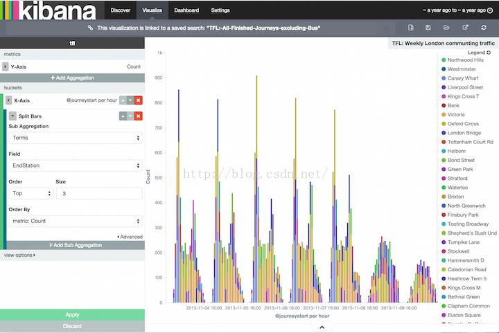
你能够在Visualization页面构建查询结果的可视化,每一个可视化界面都是和一个查询一一对应的。比如,我们可以通过上一个查询来展示一个伦敦每周通过地铁上下班的柱状图,y轴表示旅程的数量,x轴显示星期和时间。通过追加一个子聚合,我们可以看到每小时top3的目的地站。
你可以保存和分享这些形象化的图表,并且能将之结合到dashboards中,使它更容易地和某些相关的信息相互关联。比如,我们可以创建一个dashboard用于展示一些伦敦交通局数据的图表。

http://www.ruanyifeng.com/blog/2017/08/elasticsearch.html
http://blog.csdn.net/ming_311/article/details/50619804

Elasticsearch + Kibana 安装
1 安装Elasticsearch
1.1 添加普通用户
# 创建 elasticsearch 用户组
groupadd elasticsearch
#创建用户并添加密码
useradd txb_es
passwd txb_es
#创建es文件夹
mkdir -p /usr/local/es
1.2 上传文件
链接:https://pan.baidu.com/s/1bPQU9AXMmLYlil_wirpfCw
提取码:89av
获取上述elk中文件并上传至 /usr/local/es文件夹下并解压。
1.3 用户授权
usermod -G elasticsearch txb_es
chown -R txb_es /usr/local/es/elasticsearch-7.6.1/
visudo
今天关于Kibana Timelion插件如何在elasticsearch中指定字段和elasticsearch kibana配置的介绍到此结束,谢谢您的阅读,有关Building real-time dashboard applications with Apache Flink, Elasticsearch, and Kibana、docker+springboot+elasticsearch+kibana+elasticsearch-head整合(详细说明 ,看这一篇就够了)、elasticsearch + kibana、Elasticsearch + Kibana 安装等更多相关知识的信息可以在本站进行查询。
本文标签:


![[转帖]Ubuntu 安装 Wine方法(ubuntu如何安装wine)](https://www.gvkun.com/zb_users/cache/thumbs/4c83df0e2303284d68480d1b1378581d-180-120-1.jpg)